CODEX dataset

0. Environment

library(Giotto)
# STOP!
# ====== 1. set working directory ======
# For Docker, set my_working_dir to /data
my_working_dir = '/data'
# For native install users, set my_working_dir to a directory accessible by user
#my_working_dir = "/home/qzhu/Downloads"
# ====== 2. set giotto python path ======
# For Docker, set python_path to /usr/bin/python3
python_path = "/usr/bin/python3"
# For native install users, python path may be different, and may depend on whether conda or virtual environment. One can check by "reticulate::py_discover_config()" to see which python is picked up automatically. Then set python_path to what is returned by py_discover_config.
# python_path = "/usr/bin/python3"

1. Preparation steps

1.1. Dataset explanation

The CODEX data to run this tutorial can be found here Alternatively you can use the getSpatialDataset to automatically download this dataset like we do in this example.

Goltsev et al. created a multiplexed datasets of normal and lupus (MRL/lpr) murine spleens using CODEX technique. The dataset consists of 30 protein markers from 734,101 single cells. In this tutorial, 83,787 cells from sample "BALBc-3" were selected for the analysis.

1.2. Dataset download

# download data to working directory
# use method = 'wget' if wget is available. This should be much faster.
getSpatialDataset(dataset = 'codex_spleen', directory = my_working_dir, method = 'wget')

1.3. Giotto global instructions and preparations

# 1. (optional) set Giotto instructions
instrs = createGiottoInstructions(show_plot = FALSE,save_plot = TRUE,save_dir = my_working_dir,python_path = python_path)

# 2. create giotto object from provided paths ####
expr_path = fs::path(my_working_dir, "codex_BALBc_3_expression.txt.gz")
loc_path = fs::path(my_working_dir, "codex_BALBc_3_coord.txt")
meta_path = fs::path(my_working_dir, "codex_BALBc_3_annotation.txt")

2. Create Giotto object & process data

# read in data information
# expression info
codex_expression = readExprMatrix(expr_path, transpose = F)
# cell coordinate info
codex_locations = data.table::fread(loc_path)
# metadata
codex_metadata = data.table::fread(meta_path)
## stitch x.y tile coordinates to global coordinates 
xtilespan = 1344;
ytilespan = 1008;
# TODO: expand the documentation and input format of stitchTileCoordinates. Probably not enough information for new users.
stitch_file = stitchTileCoordinates(location_file = codex_metadata, Xtilespan = xtilespan, Ytilespan = ytilespan);
codex_locations = stitch_file[,.(Xcoord, Ycoord)]
# create Giotto object
codex_test <- createGiottoObject(raw_exprs = codex_expression, 
spatial_locs = codex_locations,instructions = instrs,cell_metadata = codex_metadata)
# subset Giotto object
cell_meta = pDataDT(codex_test)
cell_IDs_to_keep = cell_meta[Imaging_phenotype_cell_type != "dirt" & Imaging_phenotype_cell_type != "noid" & Imaging_phenotype_cell_type != "capsule",]$cell_ID
codex_test = subsetGiotto(codex_test, cell_ids = cell_IDs_to_keep)
## filter
codex_test <- filterGiotto(gobject = codex_test,expression_threshold = 1,gene_det_in_min_cells = 10,min_det_genes_per_cell = 2,expression_values = c('raw'),verbose = T)
codex_test <- normalizeGiotto(gobject = codex_test, scalefactor = 6000, verbose = T,log_norm = FALSE,library_size_norm = FALSE,scale_genes = FALSE, scale_cells = TRUE)
## add gene & cell statistics
codex_test <- addStatistics(gobject = codex_test,expression_values = "normalized")
## adjust expression matrix for technical or known variables
codex_test <- adjustGiottoMatrix(gobject = codex_test, 
expression_values = c('normalized'),batch_columns = NULL, 
covariate_columns = NULL,return_gobject = TRUE,update_slot = c('custom'))
## visualize
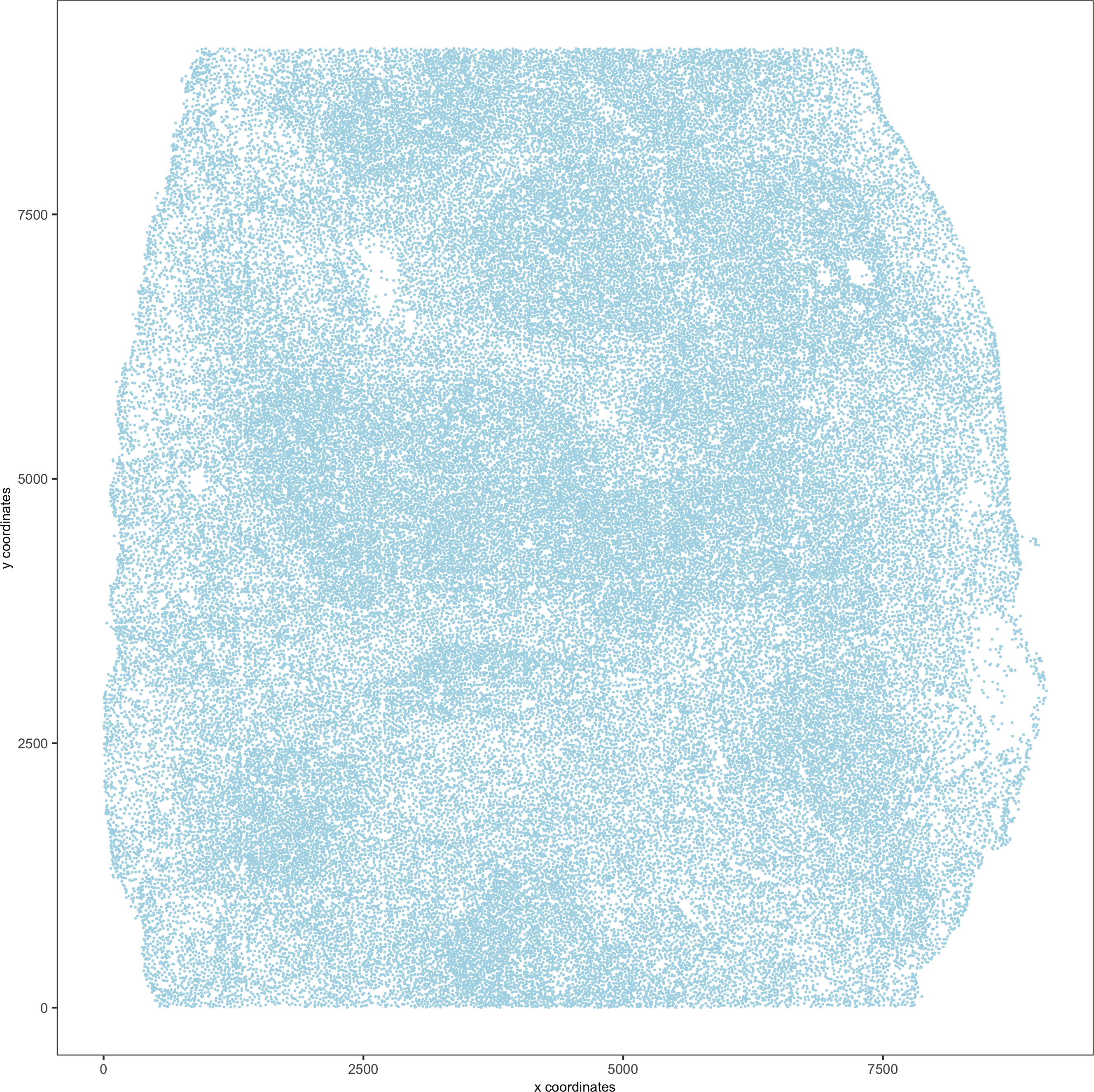
spatPlot(gobject = codex_test,point_size = 0.1, 
coord_fix_ratio = NULL,point_shape = 'no_border',save_param = list(save_name = '2_a_spatPlot'))

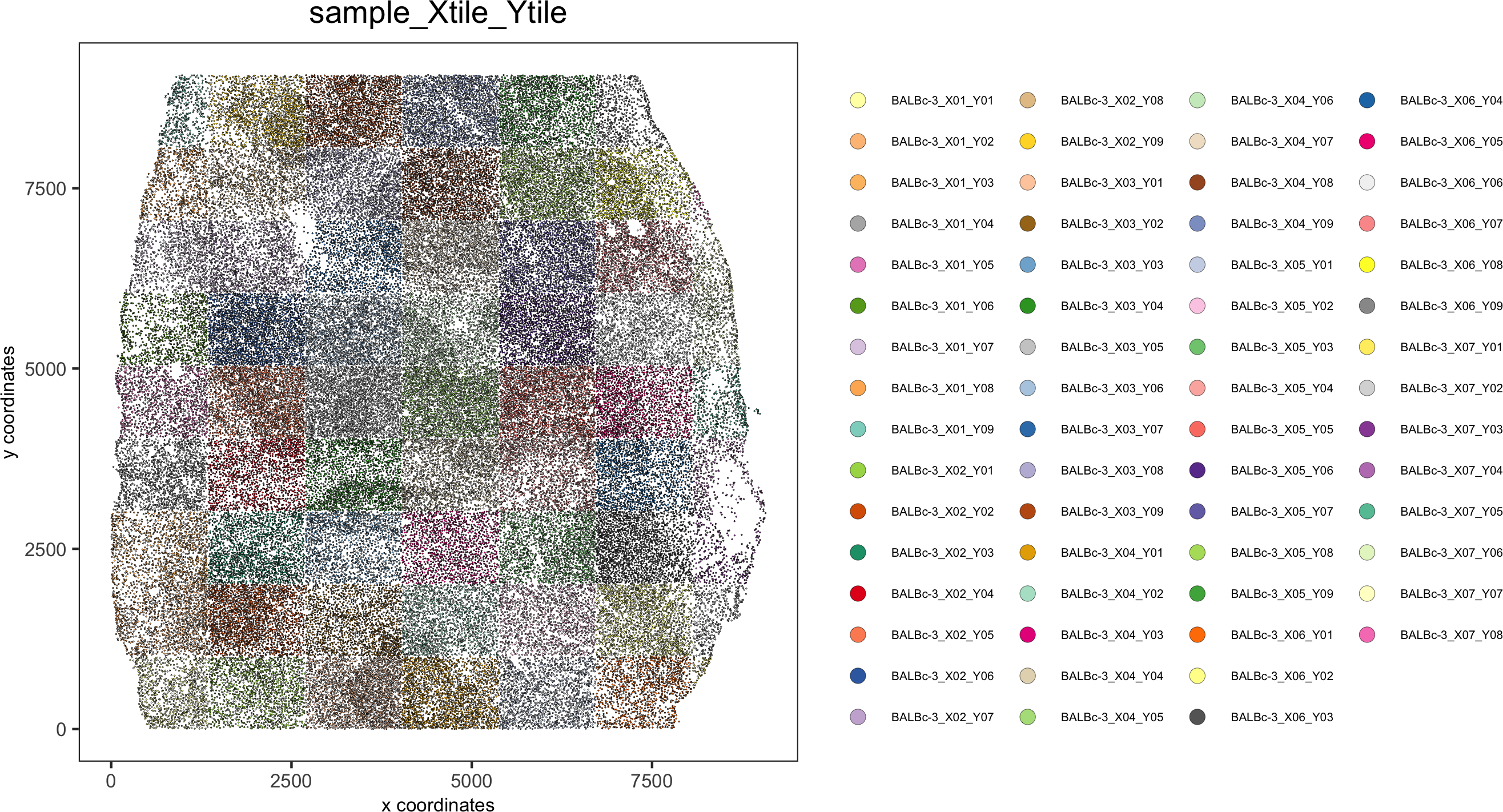
spatPlot(gobject = codex_test, point_size = 0.2,coord_fix_ratio = 1, cell_color = 'sample_Xtile_Ytile',legend_symbol_size = 3,legend_text = 5,save_param = list(save_name = '2_b_spatPlot'))

3. Dimension reduction

# use all Abs
# PCA
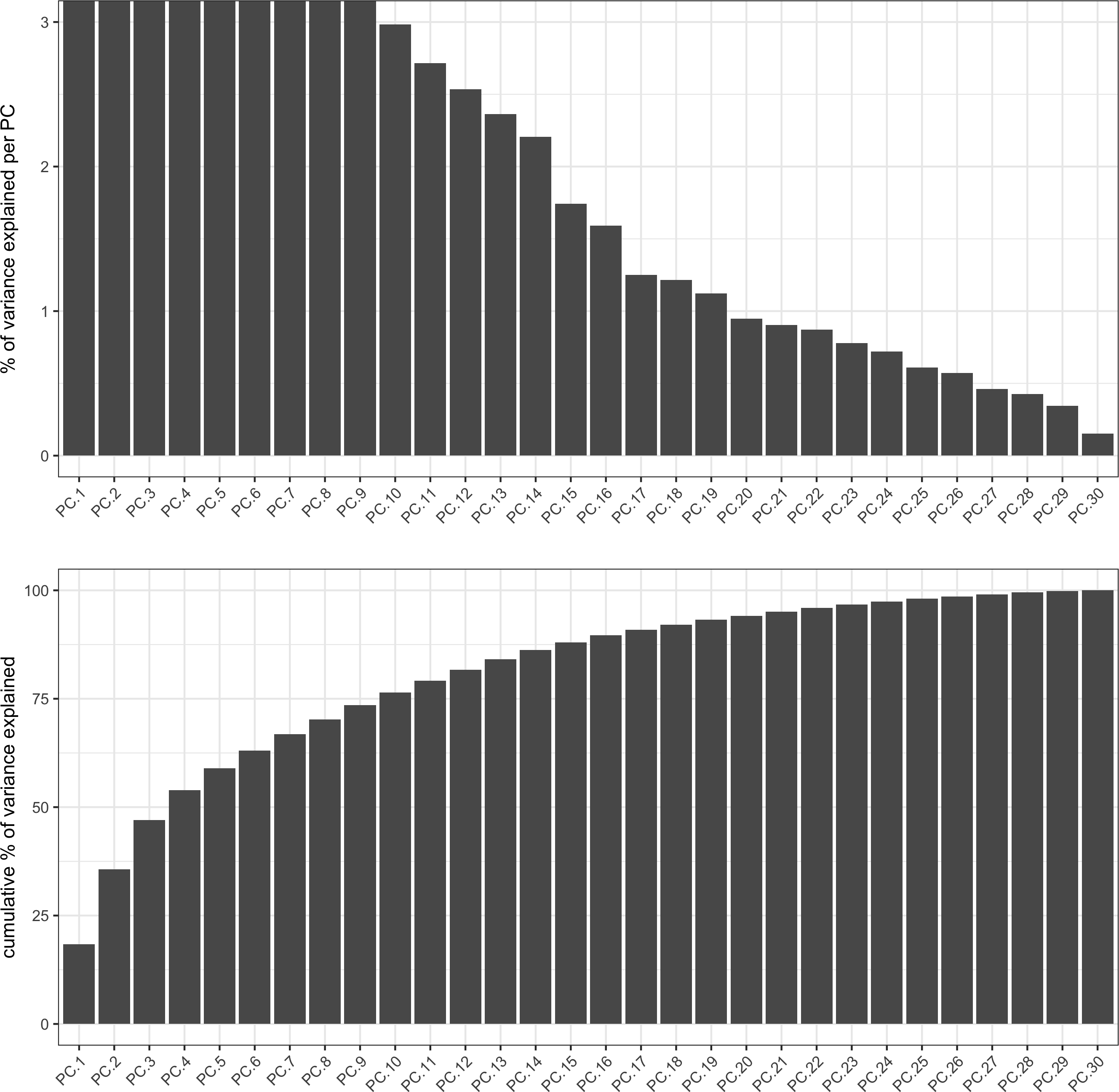
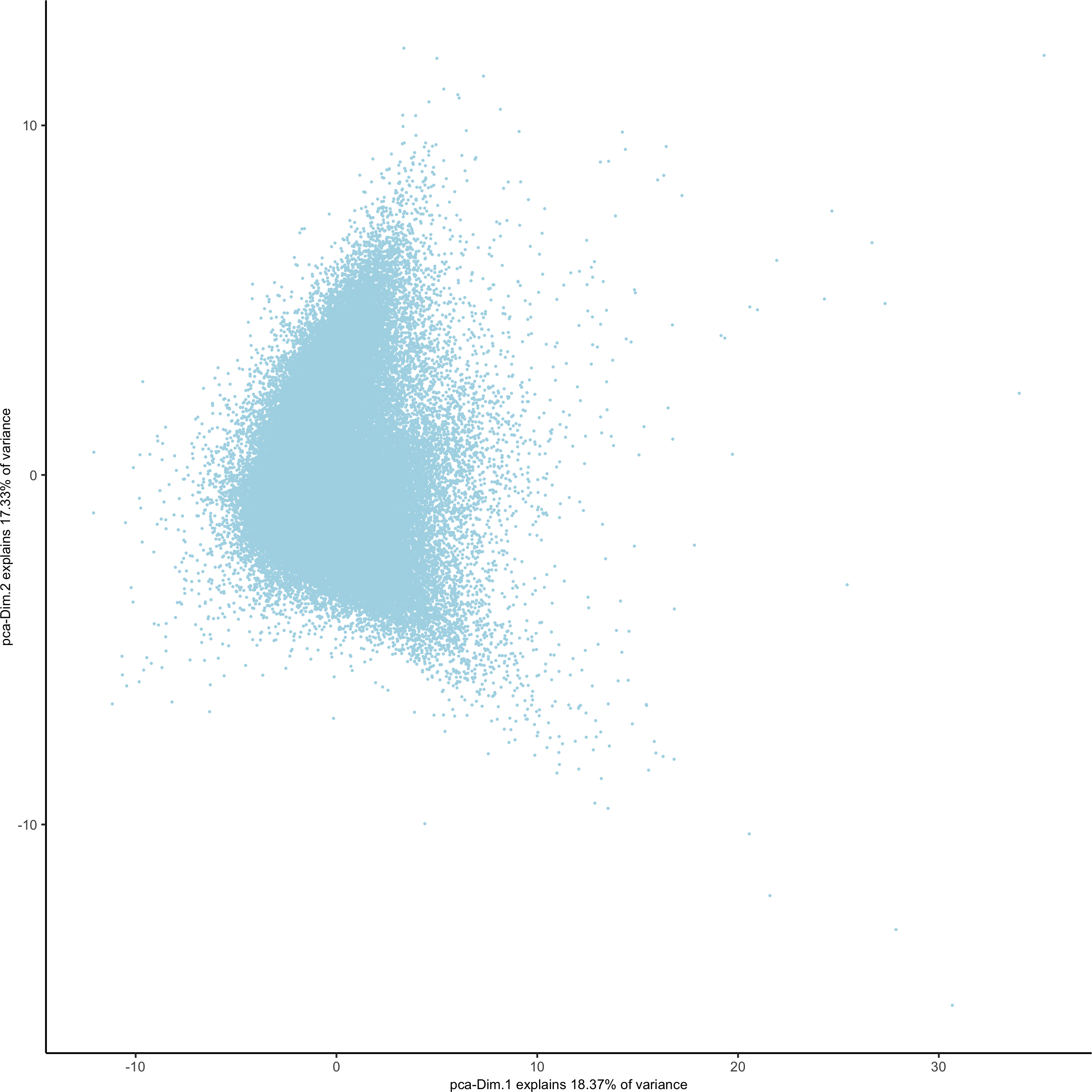
codex_test <- runPCA(gobject = codex_test, expression_values = 'normalized', scale_unit = T, method = "factominer")
signPCA(codex_test, scale_unit = T, scree_ylim = c(0, 3),save_param = list(save_name = '3_a_spatPlot'))

plotPCA(gobject = codex_test, point_shape = 'no_border', point_size = 0.2,save_param = list(save_name = '3_b_PCA'))

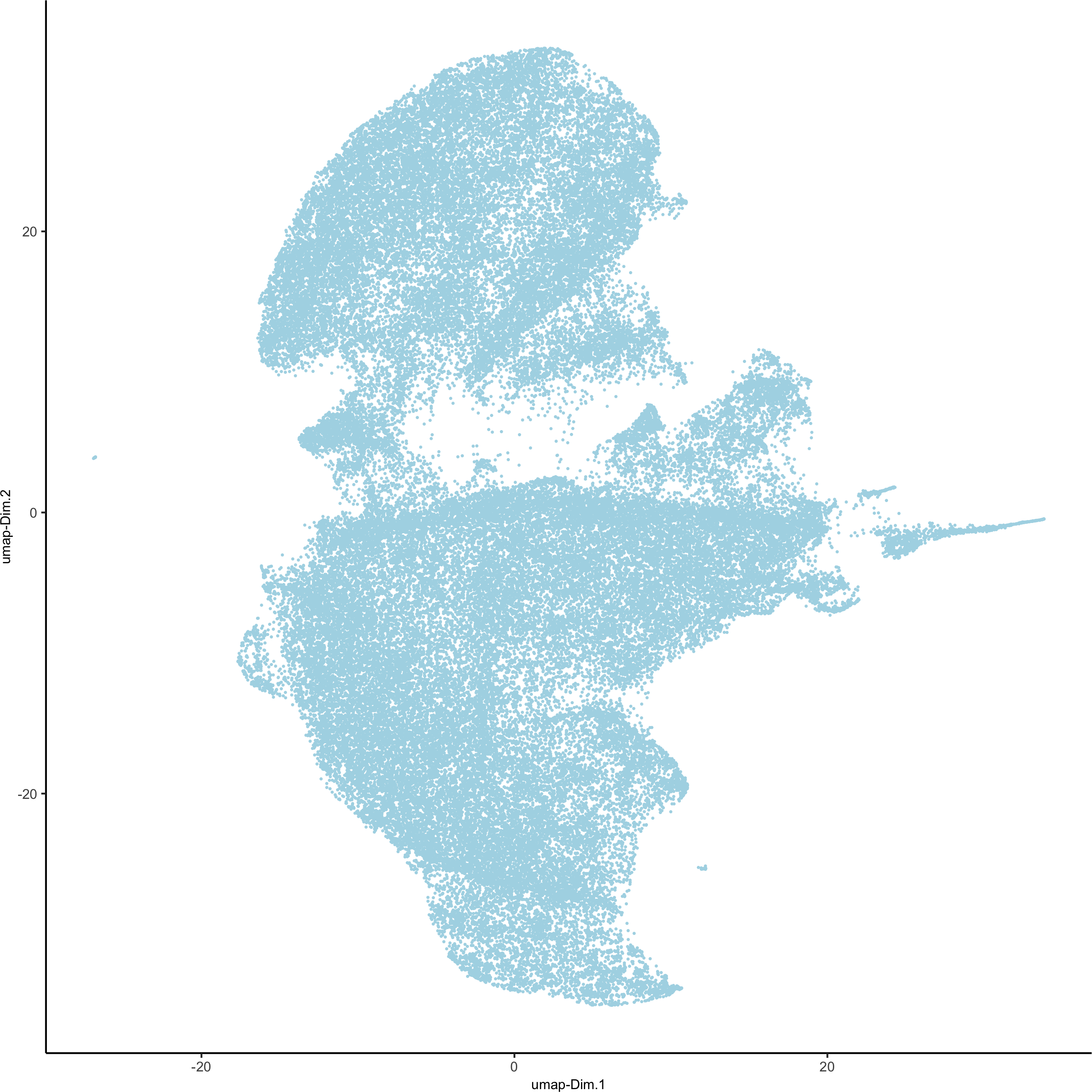
# UMAP
codex_test <- runUMAP(codex_test, dimensions_to_use = 1:14, n_components = 2, n_threads = 12)
plotUMAP(gobject = codex_test, point_shape = 'no_border', point_size = 0.2,save_param = list(save_name = '3_c_UMAP'))

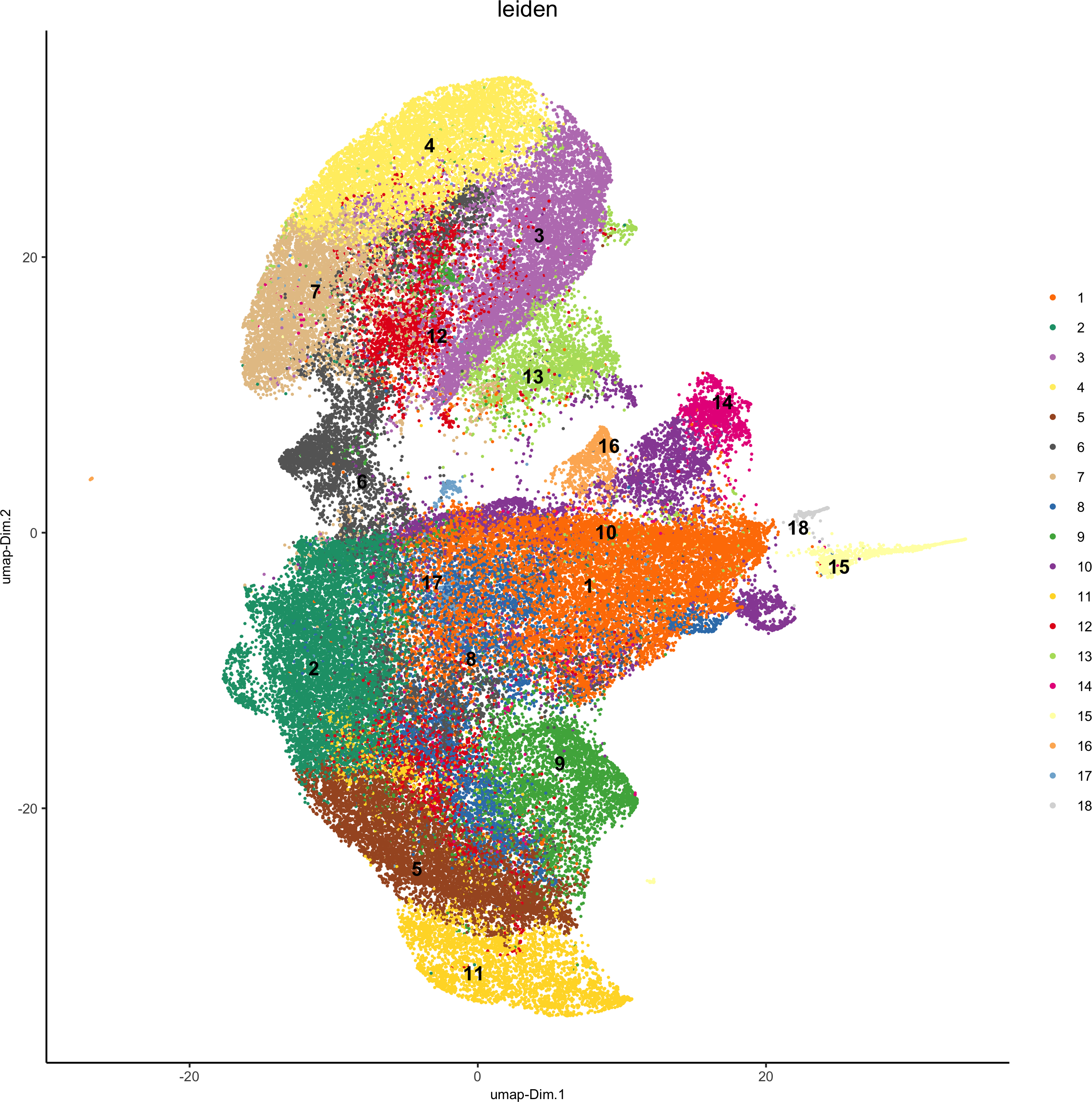
4. Cluster

## sNN network (default)
codex_test <- createNearestNetwork(gobject = codex_test, dimensions_to_use = 1:14, k = 20)
## 0.1 resolution
codex_test <- doLeidenCluster(gobject = codex_test, resolution = 0.5, n_iterations = 100, name = 'leiden',python_path = python_path)
codex_metadata = pDataDT(codex_test)
leiden_colors = Giotto:::getDistinctColors(length(unique(codex_metadata$leiden)))
names(leiden_colors) = unique(codex_metadata$leiden)
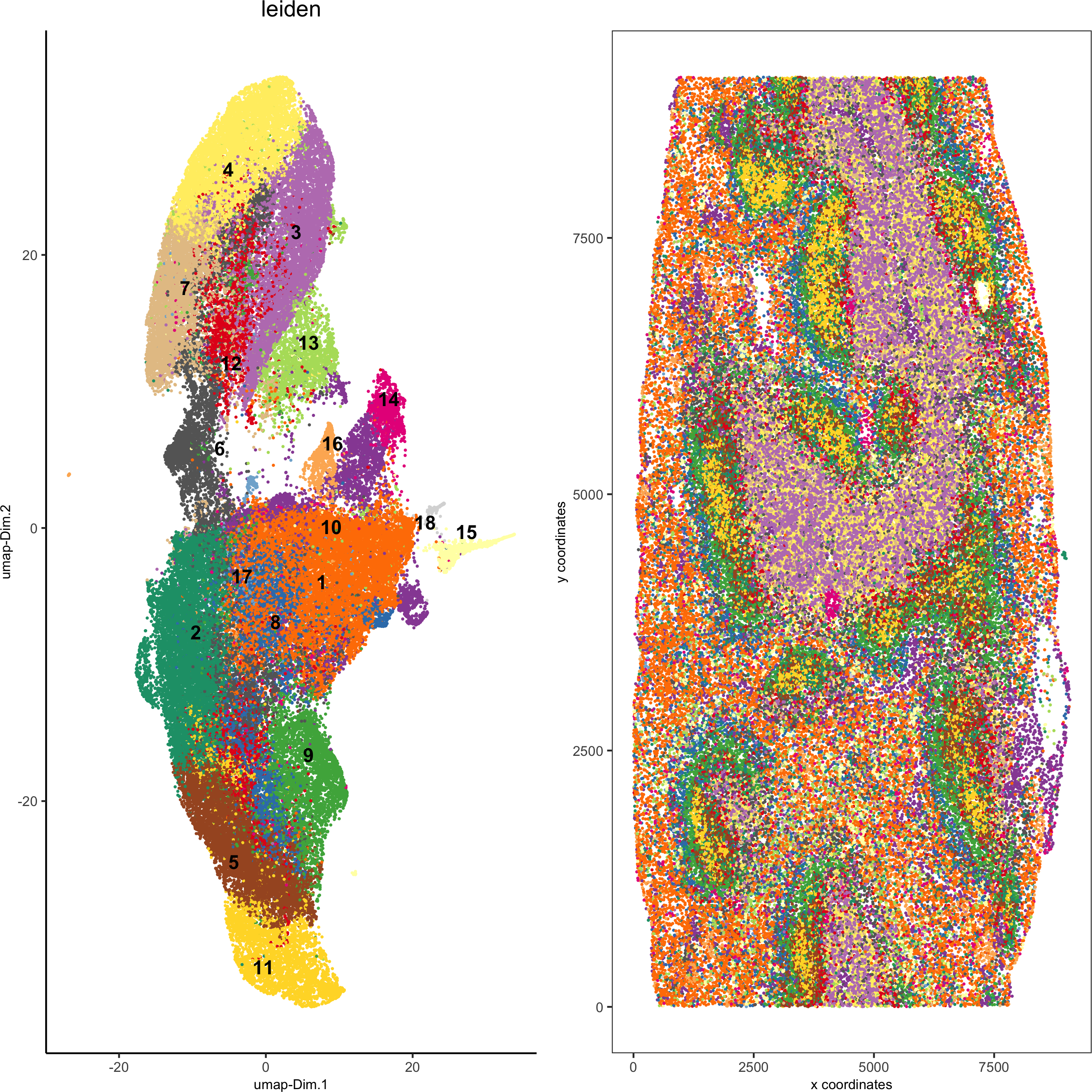
plotUMAP(gobject = codex_test, 
cell_color = 'leiden', point_shape = 'no_border', point_size = 0.2, cell_color_code = leiden_colors,save_param = list(save_name = '4_a_UMAP'))

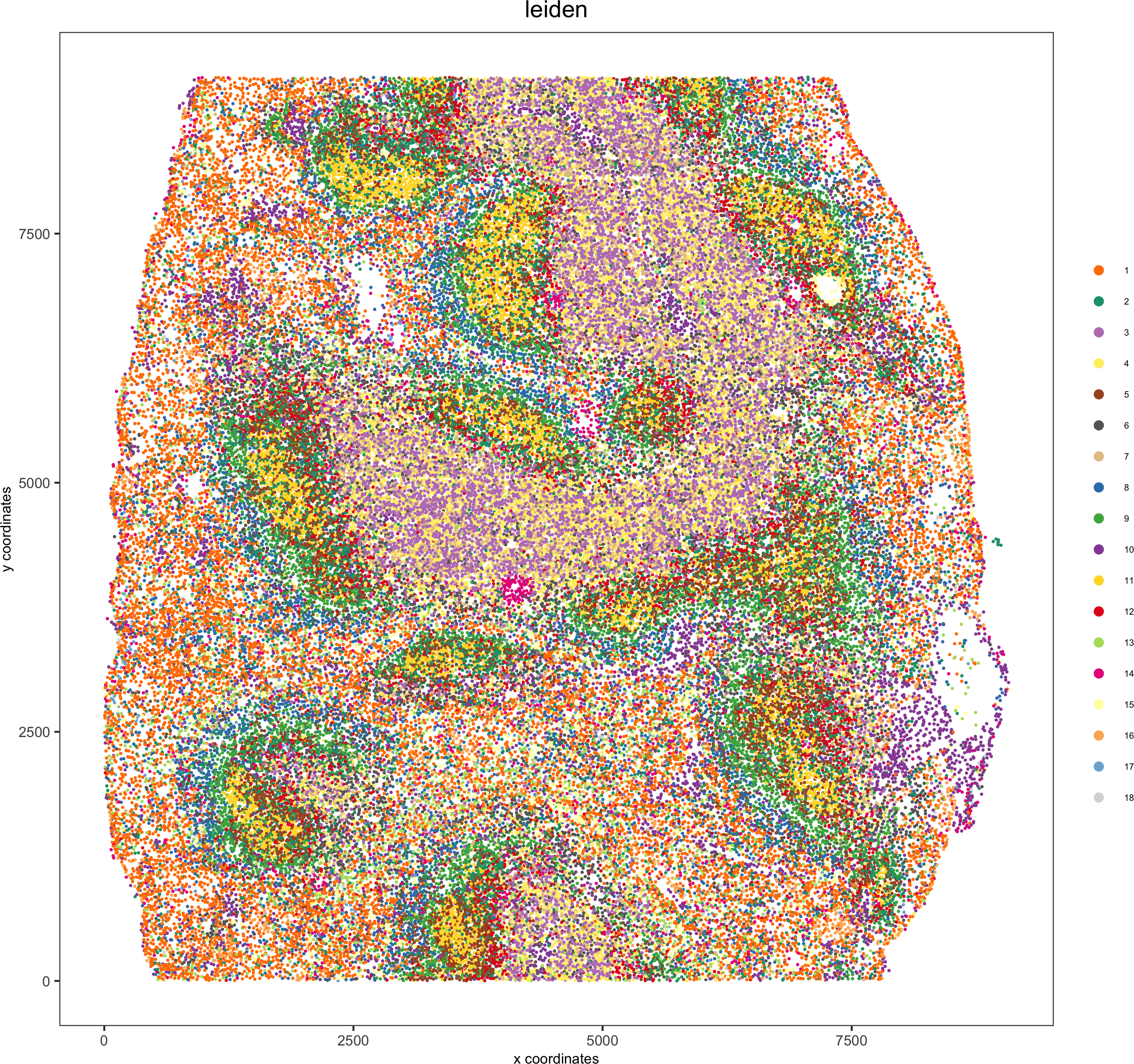
spatPlot(gobject = codex_test, cell_color = 'leiden', point_shape = 'no_border', point_size = 0.2, 
cell_color_code = leiden_colors, coord_fix_ratio = 1,label_size =2,legend_text = 5,legend_symbol_size = 2,save_param = list(save_name = '4_b_spatplot'))

5. Co-visualize

spatDimPlot2D(gobject = codex_test, cell_color = 'leiden', spat_point_shape = 'no_border', 
spat_point_size = 0.2, dim_point_shape = 'no_border', dim_point_size = 0.2, 
cell_color_code = leiden_colors,plot_alignment = c("horizontal"),save_param = list(save_name = '5_a_spatdimplot'))

6. Differential expression

# resolution 0.5
cluster_column = 'leiden'
markers_scran = findMarkers_one_vs_all(gobject=codex_test, method="scran",expression_values="norm", cluster_column=cluster_column, min_genes=3)
markergenes_scran = unique(markers_scran[, head(.SD, 5), by="cluster"][["genes"]])
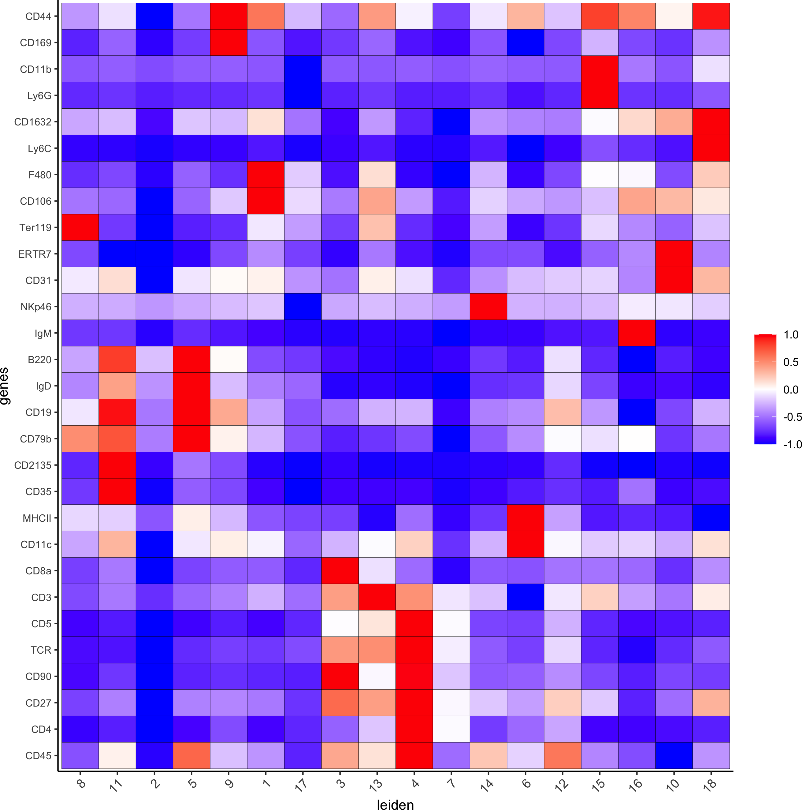
plotMetaDataHeatmap(codex_test, expression_values = "norm", metadata_cols = c(cluster_column), 
selected_genes = markergenes_scran,y_text_size = 8, show_values = 'zscores_rescaled',save_param = list(save_name = '6_a_metaheatmap'))

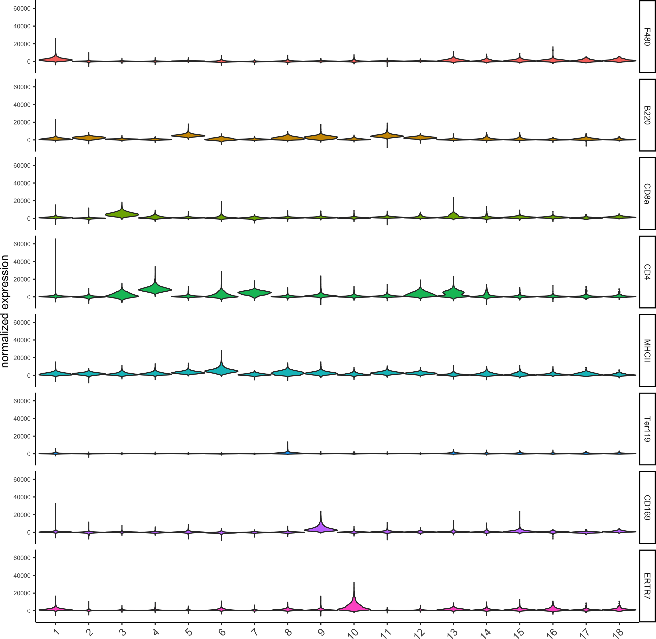
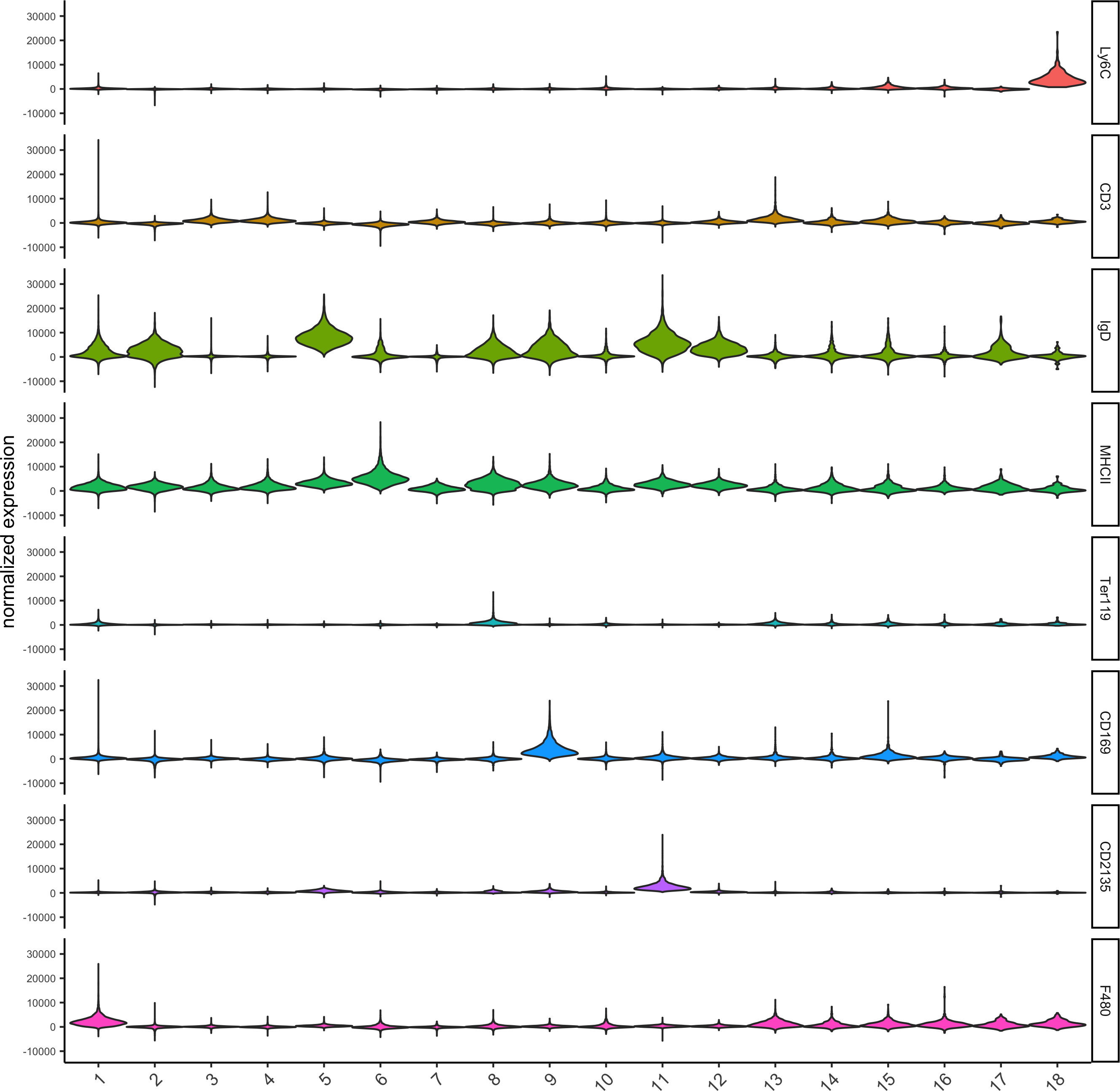
topgenes_scran = markers_scran[, head(.SD, 1), by = 'cluster']$genes
violinPlot(codex_test, genes = unique(topgenes_scran)[1:8], cluster_column = cluster_column,strip_text = 8, strip_position = 'right',save_param = list(save_name = '6_b_violinplot'))

# gini
markers_gini = findMarkers_one_vs_all(gobject=codex_test, method="gini", expression_values="norm",cluster_column=cluster_column, min_genes=5)
markergenes_gini = unique(markers_gini[, head(.SD, 5), by="cluster"][["genes"]])
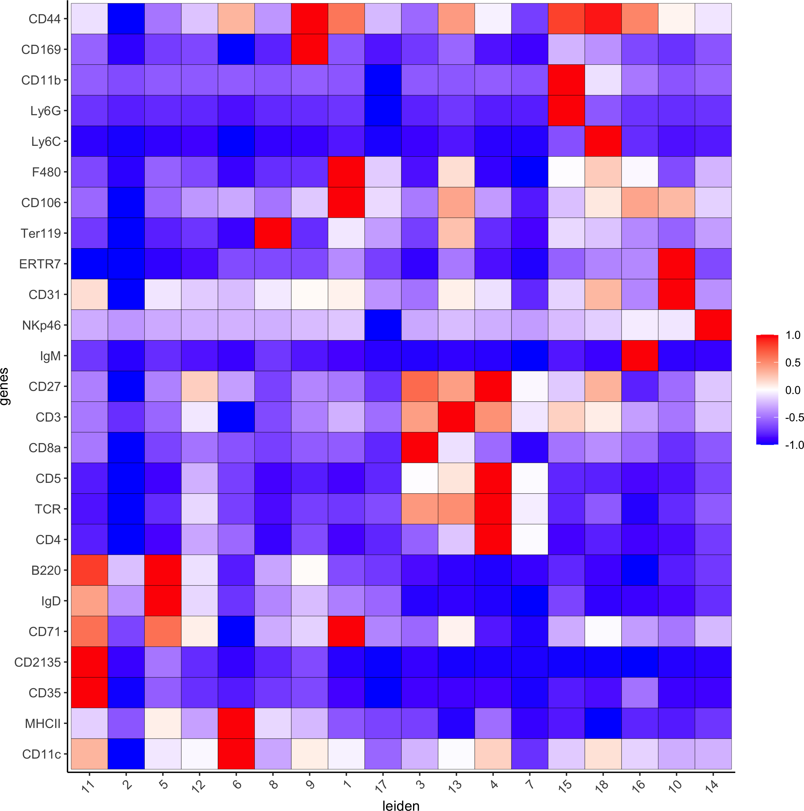
plotMetaDataHeatmap(codex_test, expression_values = "norm", 
metadata_cols = c(cluster_column), selected_genes = markergenes_gini,show_values = 'zscores_rescaled',save_param = list(save_name = '6_c_metaheatmap'))

topgenes_gini = markers_gini[, head(.SD, 1), by = 'cluster']$genes
violinPlot(codex_test, genes = unique(topgenes_gini), cluster_column = cluster_column,strip_text = 8, strip_position = 'right',save_param = list(save_name = '6_d_violinplot'))

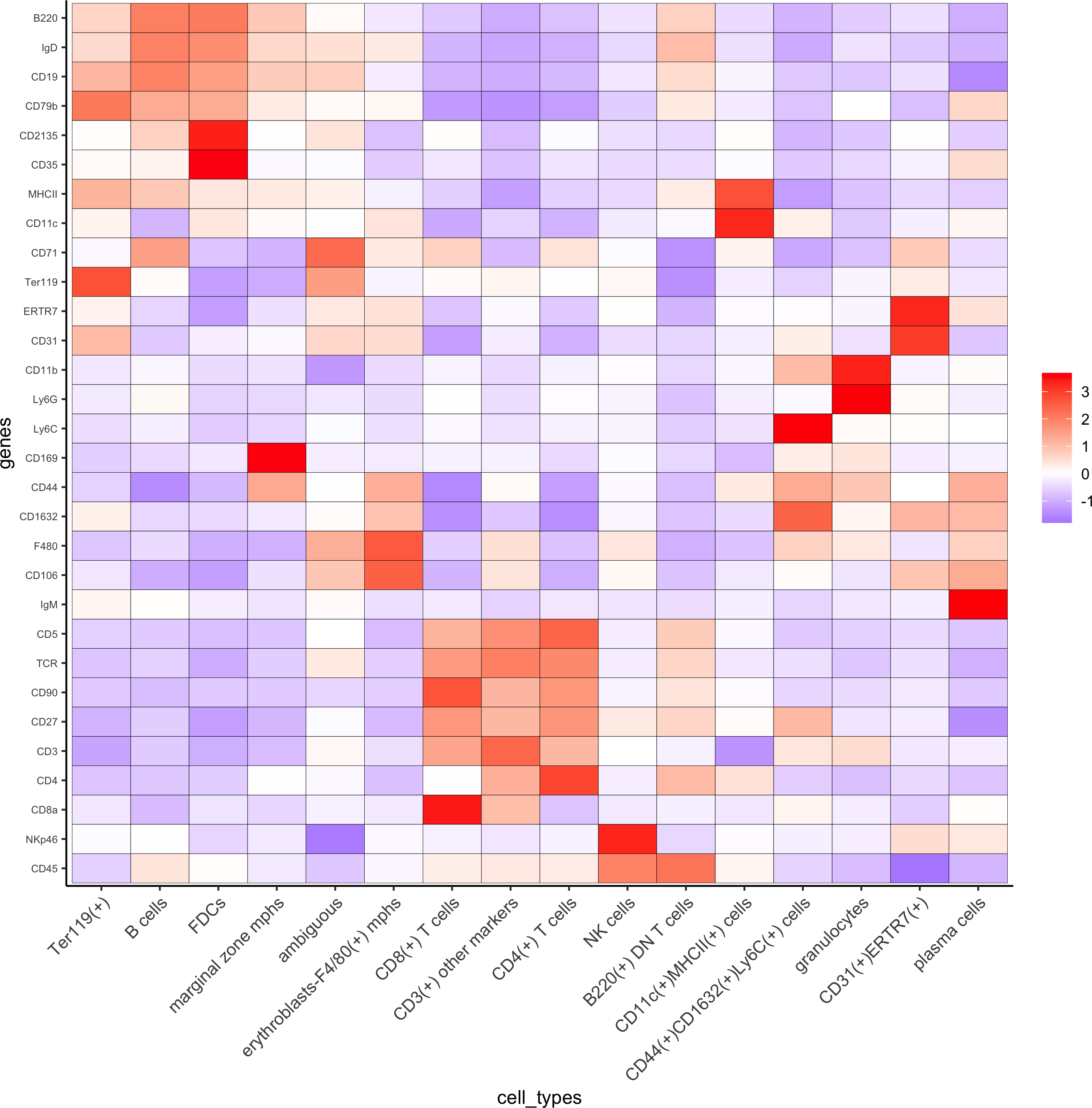
7. Cell type annotation

clusters_cell_types = c('erythroblasts-F4/80(+) mphs','B cells','CD8(+) T cells', 
'CD4(+) T cells', 'B cells','CD11c(+)MHCII(+) cells','CD4(+) T cells','Ter119(+)', 'marginal zone mphs', 
'CD31(+)ERTR7(+)', 'FDCs', 'B220(+) DN T cells','CD3(+) other markers','NK cells','granulocytes','plasma cells','ambiguous','CD44(+)CD1632(+)Ly6C(+) cells')
names(clusters_cell_types) = c(1:18)
codex_test = annotateGiotto(gobject = codex_test, annotation_vector = clusters_cell_types,cluster_column = 'leiden', name = 'cell_types')
plotMetaDataHeatmap(codex_test, expression_values = 'scaled',metadata_cols = c('cell_types'),y_text_size = 6,save_param = list(save_name = '7_a_metaheatmap'))

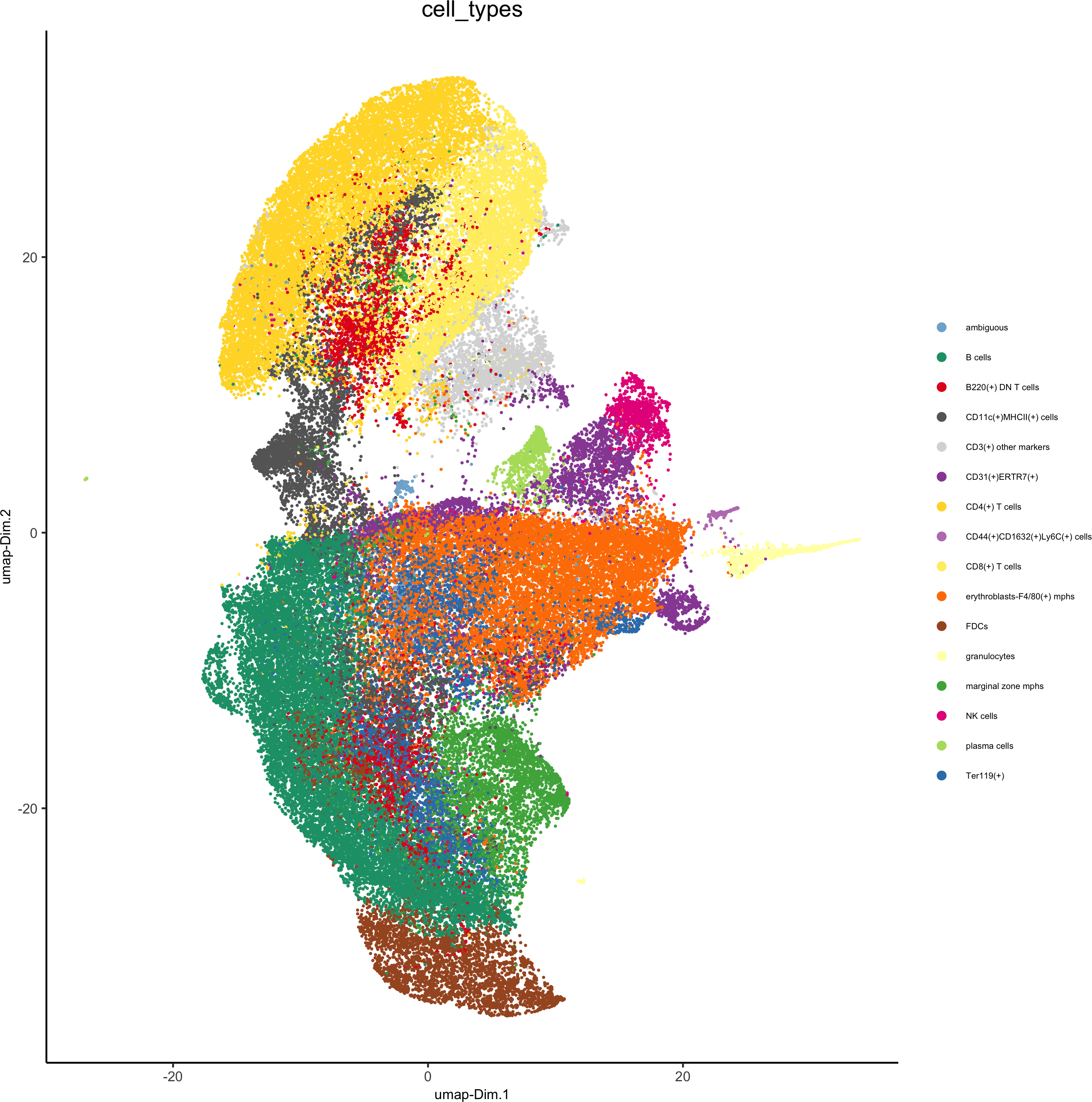
# create consistent color code
mynames = unique(pDataDT(codex_test)$cell_types)
mycolorcode = Giotto:::getDistinctColors(n = length(mynames))
names(mycolorcode) = mynames
plotUMAP(gobject = codex_test, cell_color = 'cell_types',point_shape = 'no_border',   point_size = 0.2,cell_color_code = mycolorcode,show_center_label = F,label_size =2,legend_text = 5,legend_symbol_size = 2,save_param = list(save_name = '7_b_umap'))

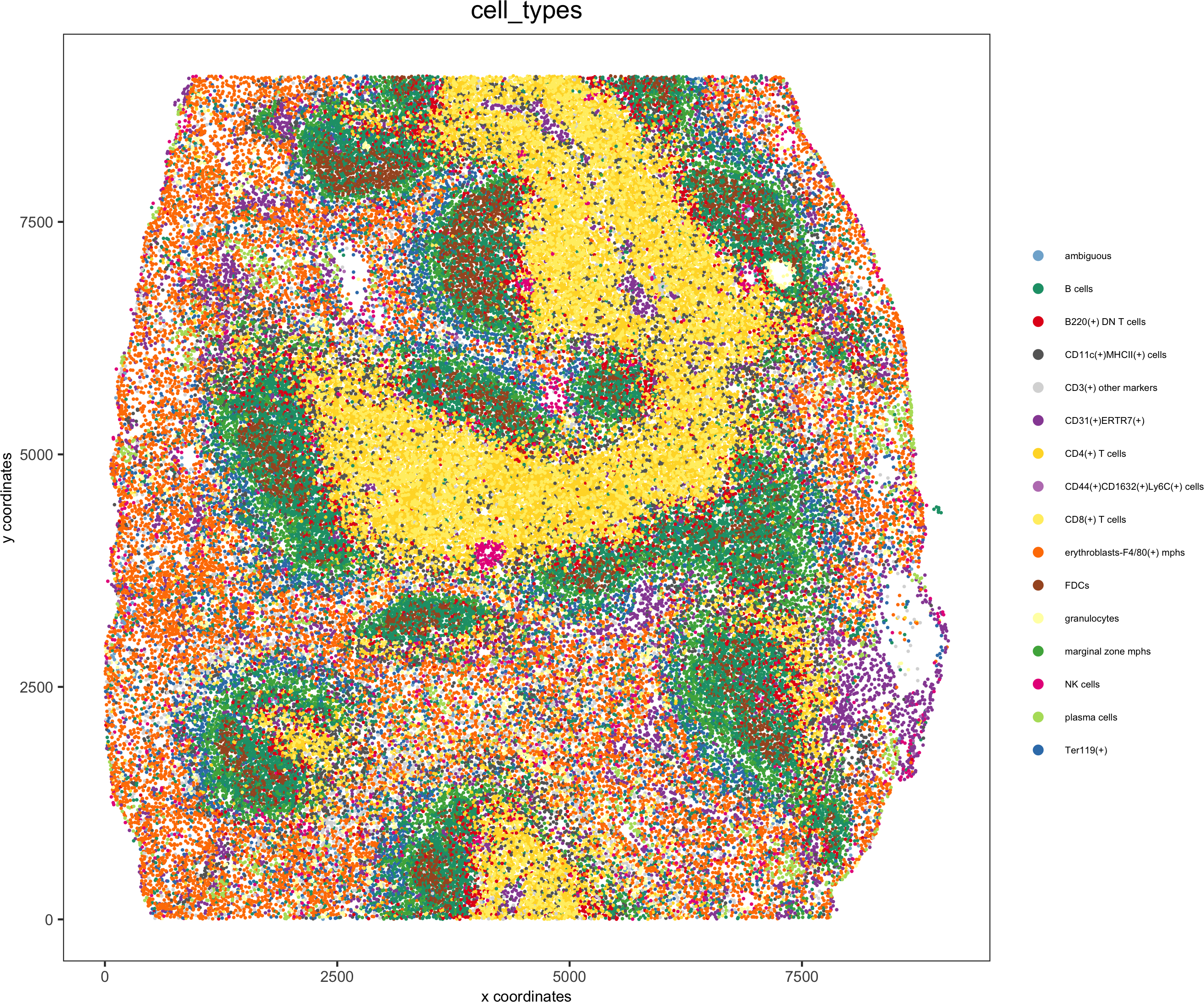
spatPlot(gobject = codex_test, cell_color = 'cell_types', point_shape = 'no_border', point_size = 0.2, 
cell_color_code = mycolorcode,coord_fix_ratio = 1,label_size =2,legend_text = 5,legend_symbol_size = 2,save_param = list(save_name = '7_c_spatplot'))

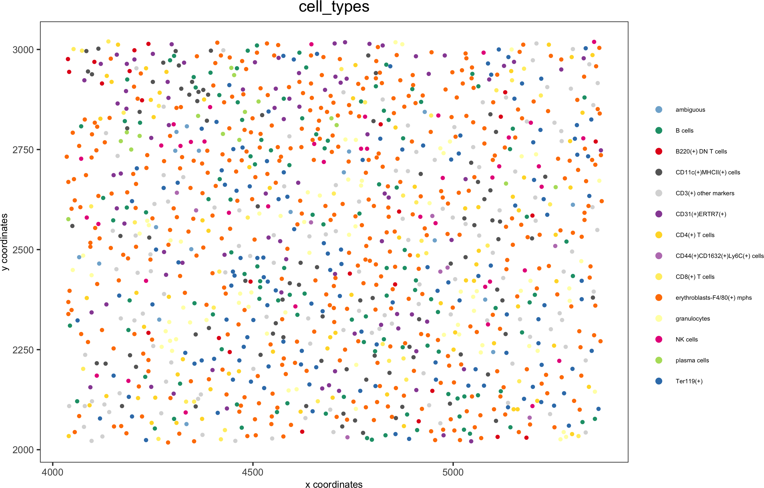
8. Visualize cell types and gene expression in selected zones

cell_metadata = pDataDT(codex_test)
subset_cell_ids = cell_metadata[sample_Xtile_Ytile=="BALBc-3_X04_Y08"]$cell_ID
codex_test_zone1 = subsetGiotto(codex_test, cell_ids = subset_cell_ids)
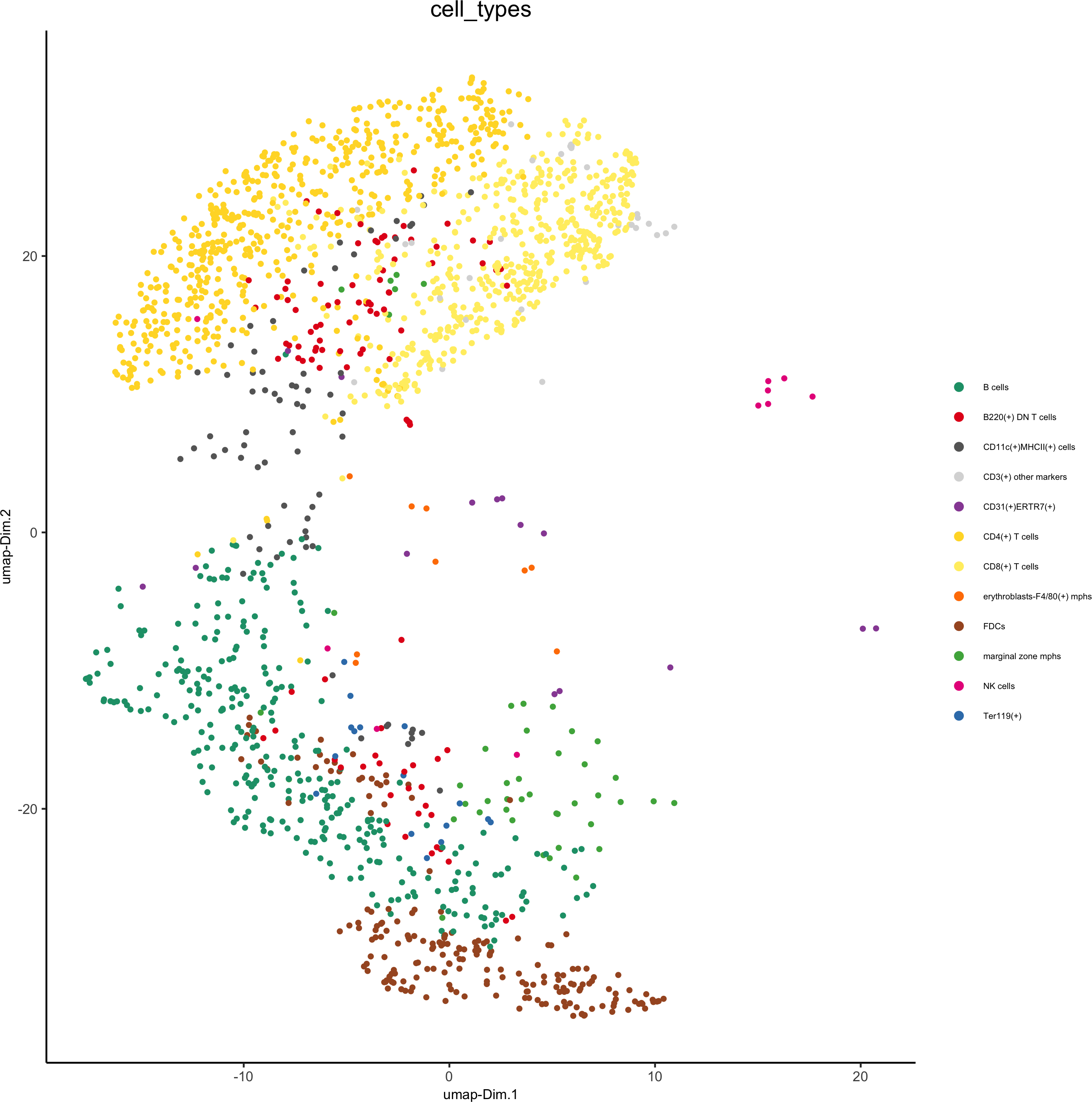
plotUMAP(gobject = codex_test_zone1, 
cell_color = 'cell_types', point_shape = 'no_border',   point_size = 1,cell_color_code = mycolorcode,show_center_label = F,label_size =2,legend_text = 5,legend_symbol_size = 2,save_param = list(save_name = '8_a_umap'))

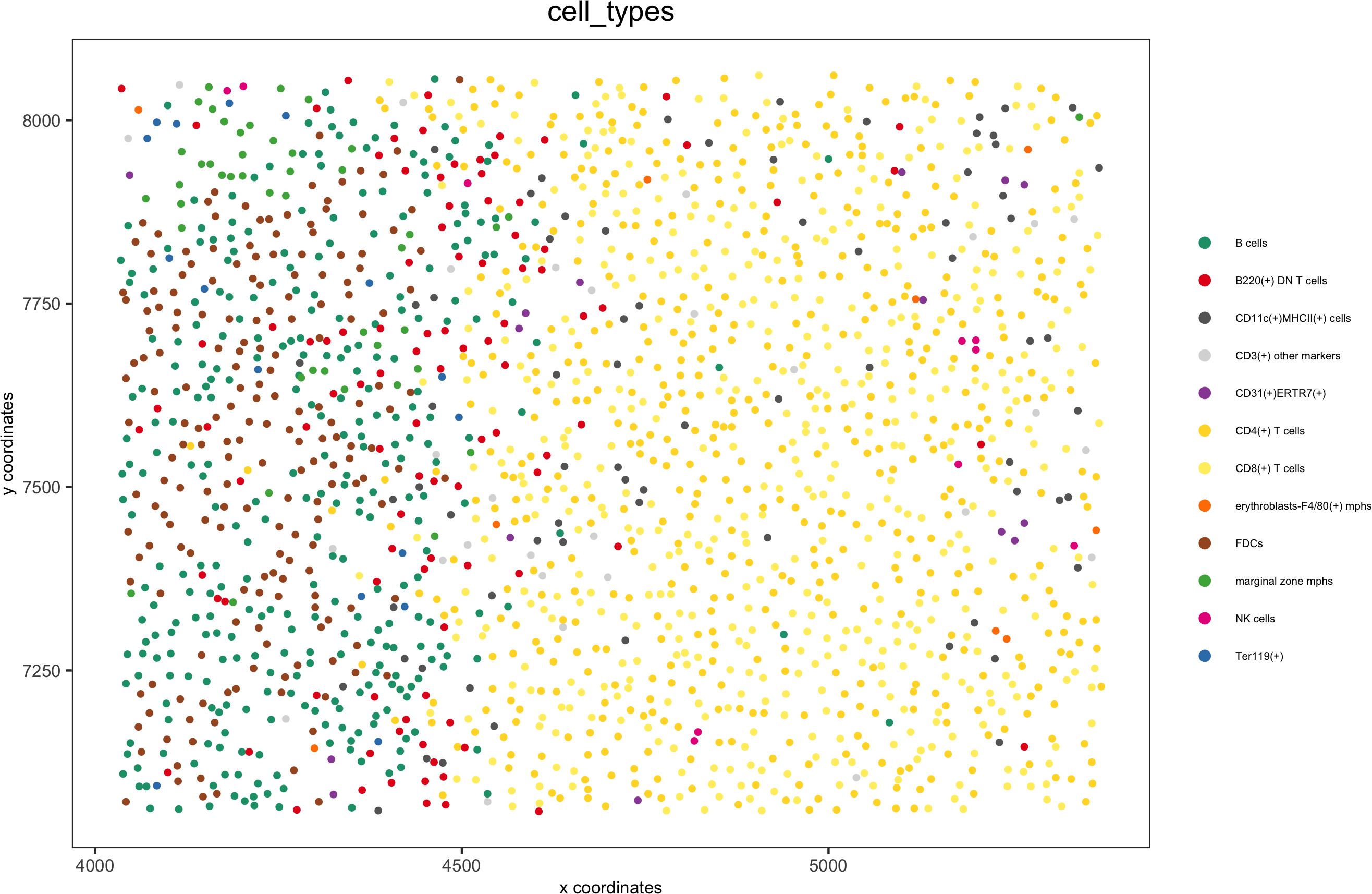
spatPlot(gobject = codex_test_zone1, 
cell_color = 'cell_types', point_shape = 'no_border', point_size = 1, 
cell_color_code = mycolorcode,coord_fix_ratio = 1,label_size =2,legend_text = 5,legend_symbol_size = 2,save_param = list(save_name = '8_b_spatplot'))

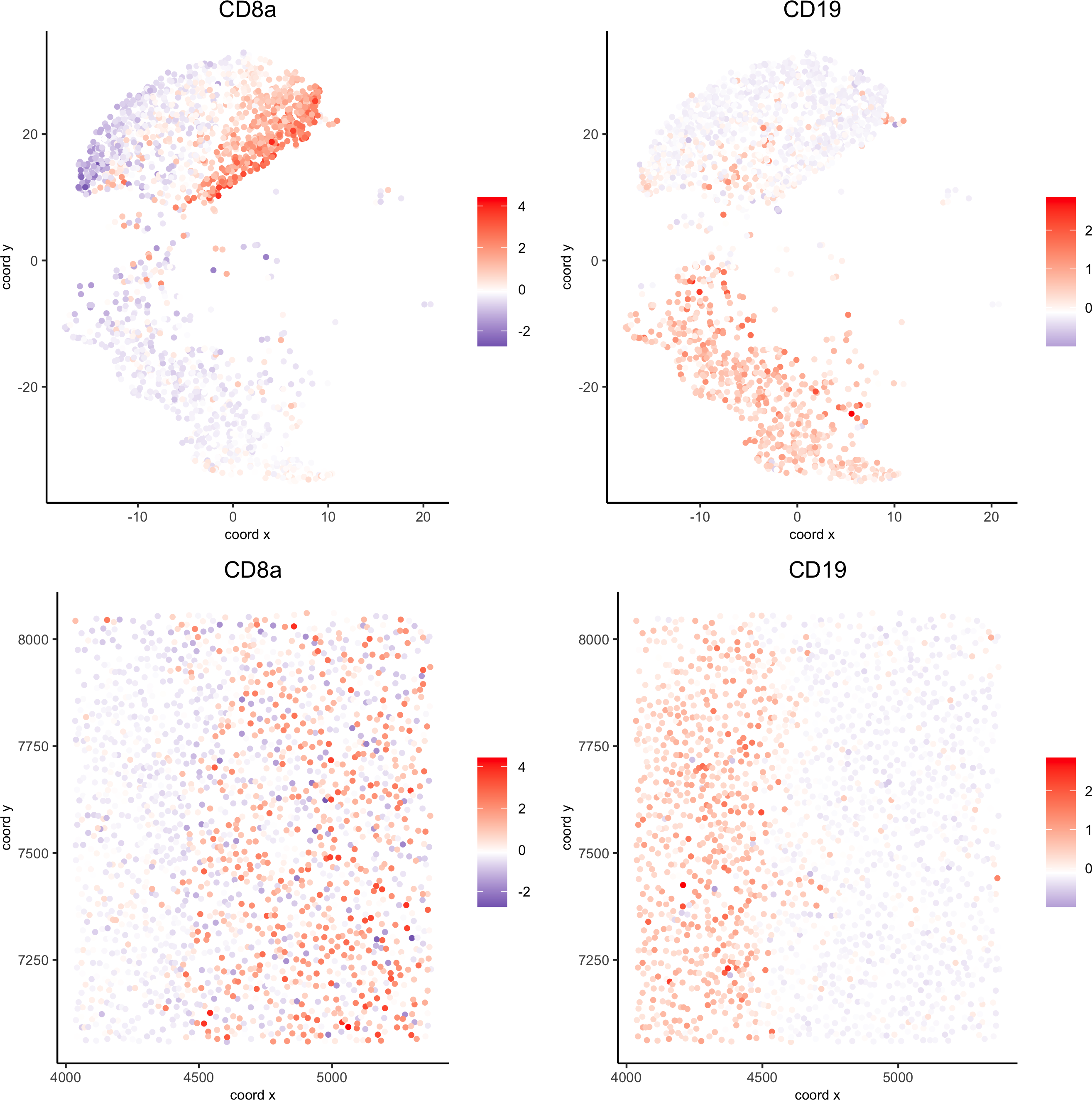
spatDimGenePlot(codex_test_zone1, 
expression_values = 'scaled',genes = c("CD8a","CD19"),spat_point_shape = 'no_border',dim_point_shape = 'no_border',cell_color_gradient = c("darkblue", "white", "red"),save_param = list(save_name = '8_c_spatdimplot'))

cell_metadata = pDataDT(codex_test)
subset_cell_ids = cell_metadata[sample_Xtile_Ytile=="BALBc-3_X04_Y03"]$cell_ID
codex_test_zone2 = subsetGiotto(codex_test, cell_ids = subset_cell_ids)
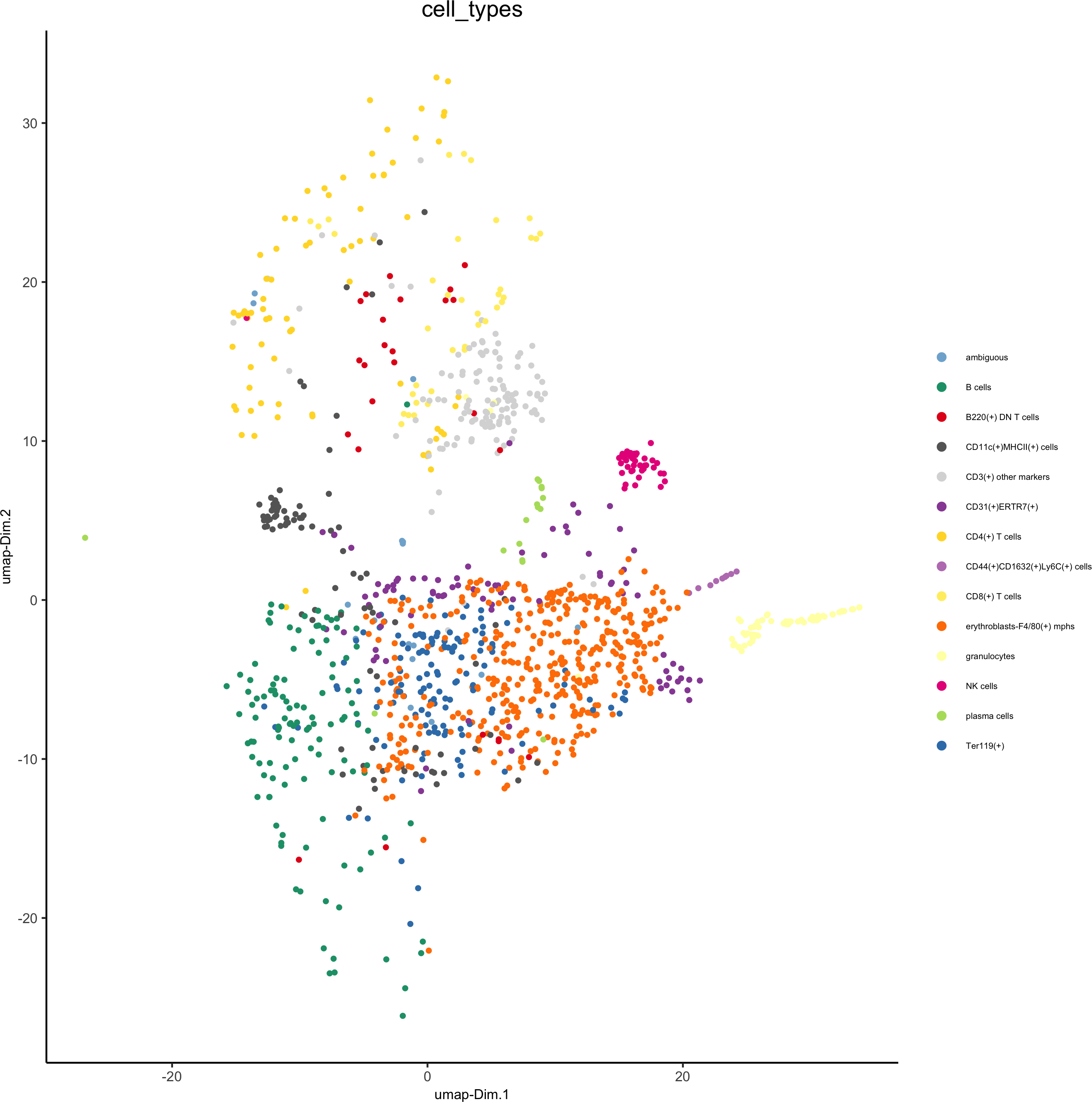
plotUMAP(gobject = codex_test_zone2, cell_color = 'cell_types',point_shape = 'no_border',   point_size = 1,cell_color_code = mycolorcode,show_center_label = F,label_size =2,legend_text = 5,legend_symbol_size = 2,save_param = list(save_name = '8_d_umap'))

spatPlot(gobject = codex_test_zone2, cell_color = 'cell_types', point_shape = 'no_border', point_size = 1, 
cell_color_code = mycolorcode,coord_fix_ratio = 1,label_size =2,legend_text = 5,legend_symbol_size = 2,save_param = list(save_name = '8_e_spatPlot'))

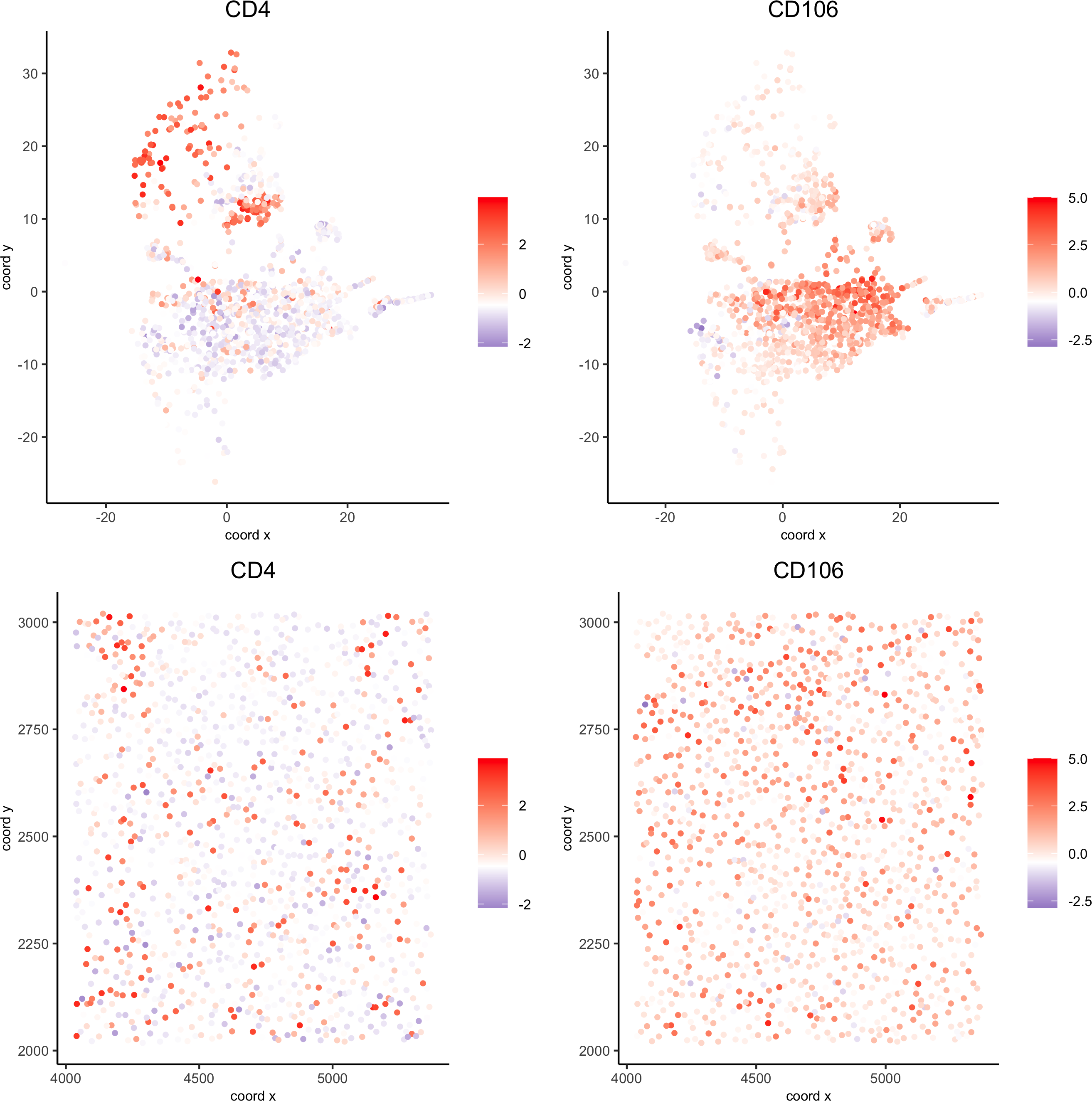
spatDimGenePlot(codex_test_zone2, 
expression_values = 'scaled',genes = c("CD4", "CD106"),spat_point_shape = 'no_border',dim_point_shape = 'no_border',cell_color_gradient = c("darkblue", "white", "red"),save_param = list(save_name = '8_f_spatdimgeneplot'))