seqFISH+ dataset

0. Environment

library(Giotto)
# STOP!
# ====== 1. set working directory ======
# For Docker, set my_working_dir to /data
my_working_dir = '/data'
# For native install users, set my_working_dir to a directory accessible by user
#my_working_dir = "/home/qzhu/Downloads"
# ====== 2. set giotto python path ======
# For Docker, set python_path to /usr/bin/python3
python_path = "/usr/bin/python3"
# For native install users, python path may be different, and may depend on whether conda or virtual environment. One can check by "reticulate::py_discover_config()" to see which python is picked up automatically. Then set python_path to what is returned by py_discover_config.
# python_path = "/usr/bin/python3"

1. Preparation steps

1.1. Dataset downloading

# download data to working directory ####
# if wget is installed, set method = 'wget'
getSpatialDataset(dataset = 'seqfish_SS_cortex', directory = my_working_dir, method = 'wget')

1.2. Giotto global instructions, stitching coordinates

# 1. (optional) set Giotto instructions
instrs = createGiottoInstructions(save_plot = TRUE,show_plot = FALSE,save_dir = my_working_dir,python_path = python_path)
# 2. create giotto object from provided paths ####
expr_path = fs::path(my_working_dir, "cortex_svz_expression.txt")
loc_path = fs::path(my_working_dir, "cortex_svz_centroids_coord.txt")
meta_path = fs::path(my_working_dir, "cortex_svz_centroids_annot.txt")
# 3. This dataset contains multiple field of views which need to be stitched together
## first merge location and additional metadata
SS_locations = data.table::fread(loc_path)
cortex_fields = data.table::fread(meta_path)
SS_loc_annot = data.table::merge.data.table(SS_locations, cortex_fields, by = 'ID')
SS_loc_annot[, ID := factor(ID, levels = paste0('cell_',1:913))]
data.table::setorder(SS_loc_annot, ID)
## create file with offset information
my_offset_file = data.table::data.table(field = c(0, 1, 2, 3, 4, 5, 6), x_offset = c(0, 1654.97, 1750.75, 1674.35, 675.5, 2048, 675), y_offset = c(0, 0, 0, 0, -1438.02, -1438.02, 0))
## create a stitch file
stitch_file = stitchFieldCoordinates(location_file = SS_loc_annot,offset_file = my_offset_file,cumulate_offset_x = T,cumulate_offset_y = F,field_col = 'FOV', reverse_final_x = F, reverse_final_y = T)
stitch_file = stitch_file[,.(ID, X_final, Y_final)]
my_offset_file = my_offset_file[,.(field, x_offset_final, y_offset_final)]

1.3. Create Giotto Object

SS_seqfish <- createGiottoObject(raw_exprs = expr_path,spatial_locs = stitch_file,offset_file = my_offset_file, instructions = instrs)

1.4. Filtering, normalization

SS_seqfish = addCellMetadata(SS_seqfish,new_metadata = cortex_fields,by_column = T,column_cell_ID = 'ID')
cell_metadata = pDataDT(SS_seqfish)
cortex_cell_ids = cell_metadata[FOV %in% 0:4]$cell_ID
SS_seqfish = subsetGiotto(SS_seqfish, cell_ids = cortex_cell_ids)
SS_seqfish <- filterGiotto(gobject = SS_seqfish,expression_threshold = 1,gene_det_in_min_cells = 10,min_det_genes_per_cell = 10, expression_values = c('raw'),verbose = T)
## normalize
SS_seqfish <- normalizeGiotto(gobject = SS_seqfish, scalefactor = 6000, verbose = T)
## add gene & cell statistics
SS_seqfish <- addStatistics(gobject = SS_seqfish)
## adjust expression matrix for technical or known variables
SS_seqfish <- adjustGiottoMatrix(gobject = SS_seqfish, expression_values = c('normalized'),batch_columns = NULL, covariate_columns = c('nr_genes', 'total_expr'),return_gobject = TRUE,update_slot = c('custom'))

## visualize
spatPlot(gobject = SS_seqfish, save_param = list(save_name = '2_spatplot'))

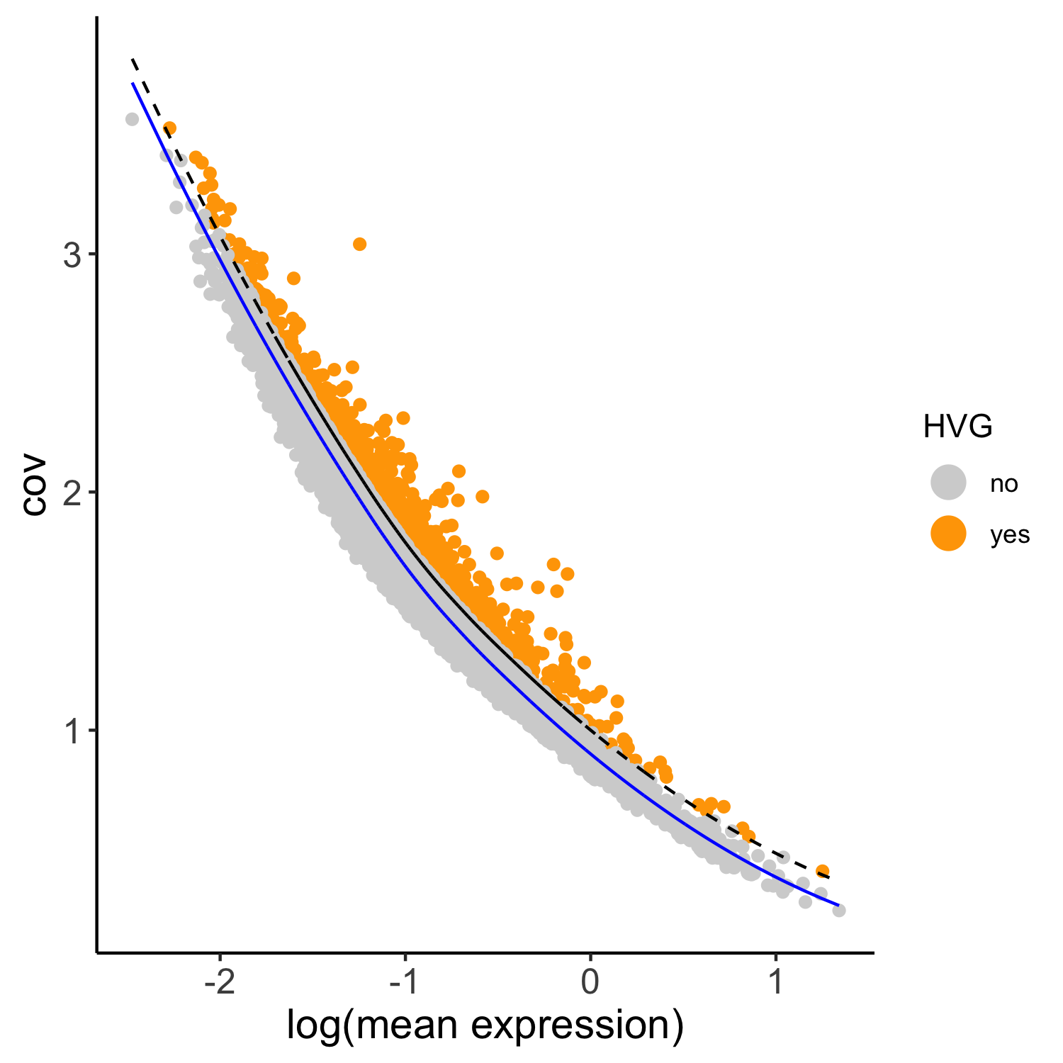
2. Highly variable genes (HVG)

SS_seqfish <- calculateHVG(gobject = SS_seqfish, method = 'cov_loess', difference_in_cov = 0.1, save_param = list(save_name = '3_a_HVGplot', base_height = 5, base_width = 5))
## select genes based on HVG and gene statistics, both found in gene metadata
gene_metadata = fDataDT(SS_seqfish)
featgenes = gene_metadata[hvg == 'yes' & perc_cells > 4 & mean_expr_det > 0.5]$gene_ID

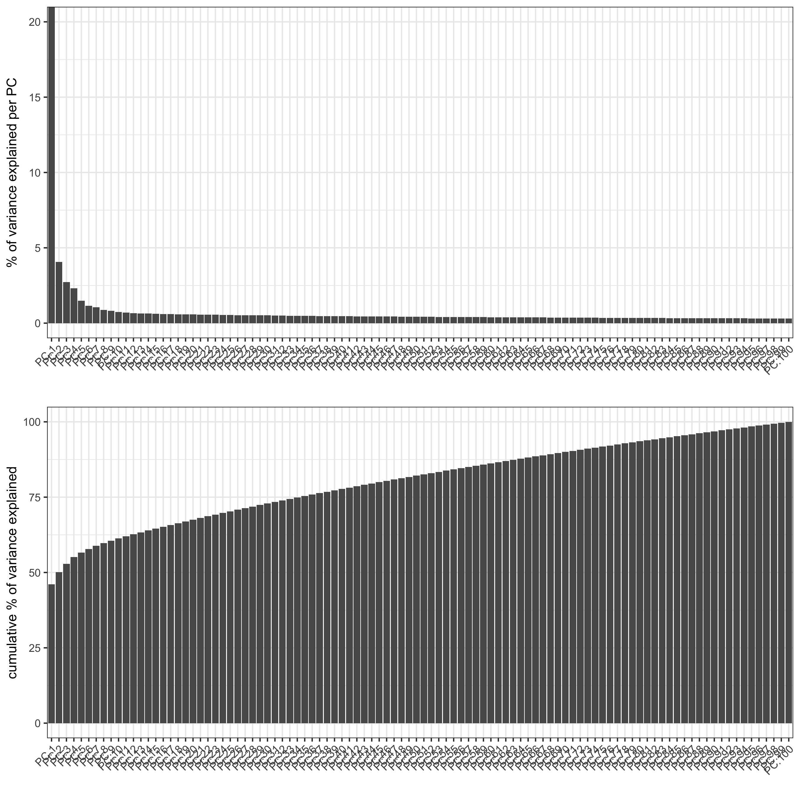
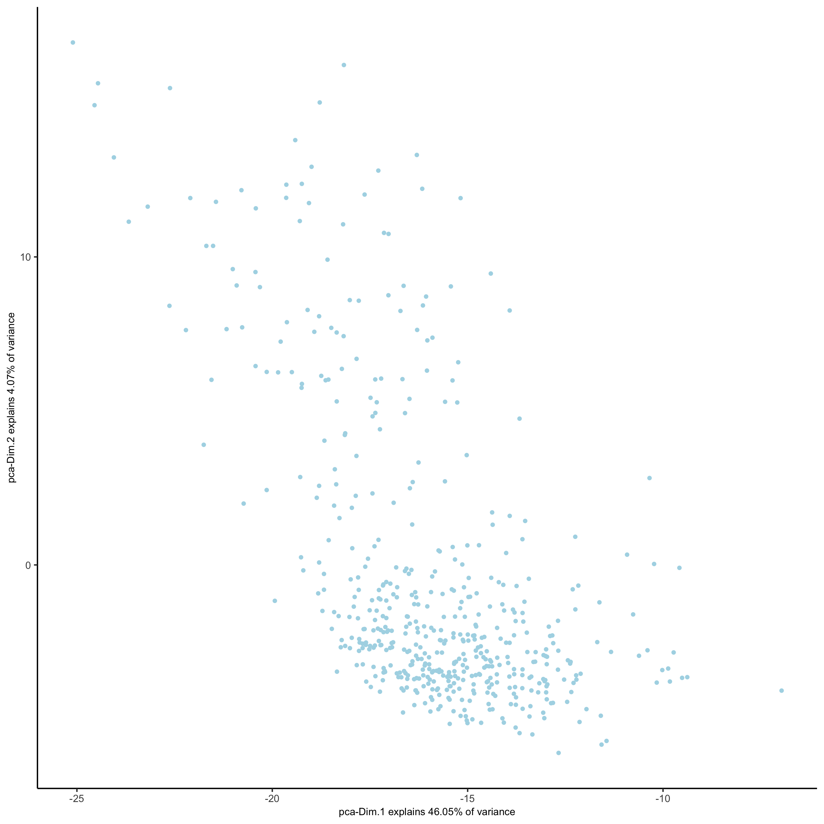
3. PCA, UMAP, tSNE

# runPCA: normal and recommended usage, set center = T:
# SS_seqfish <- runPCA(gobject = SS_seqfish, genes_to_use = featgenes, scale_unit = F, center = T)
# center=F for compatibility reason (with paper and previous Giotto version):
SS_seqfish <- runPCA(gobject = SS_seqfish, genes_to_use = featgenes, scale_unit = F, center = F)
screePlot(SS_seqfish, save_param = list(save_name = '3_b_screeplot'))
plotPCA(gobject = SS_seqfish,save_param = list(save_name = '3_c_PCA_reduction'))
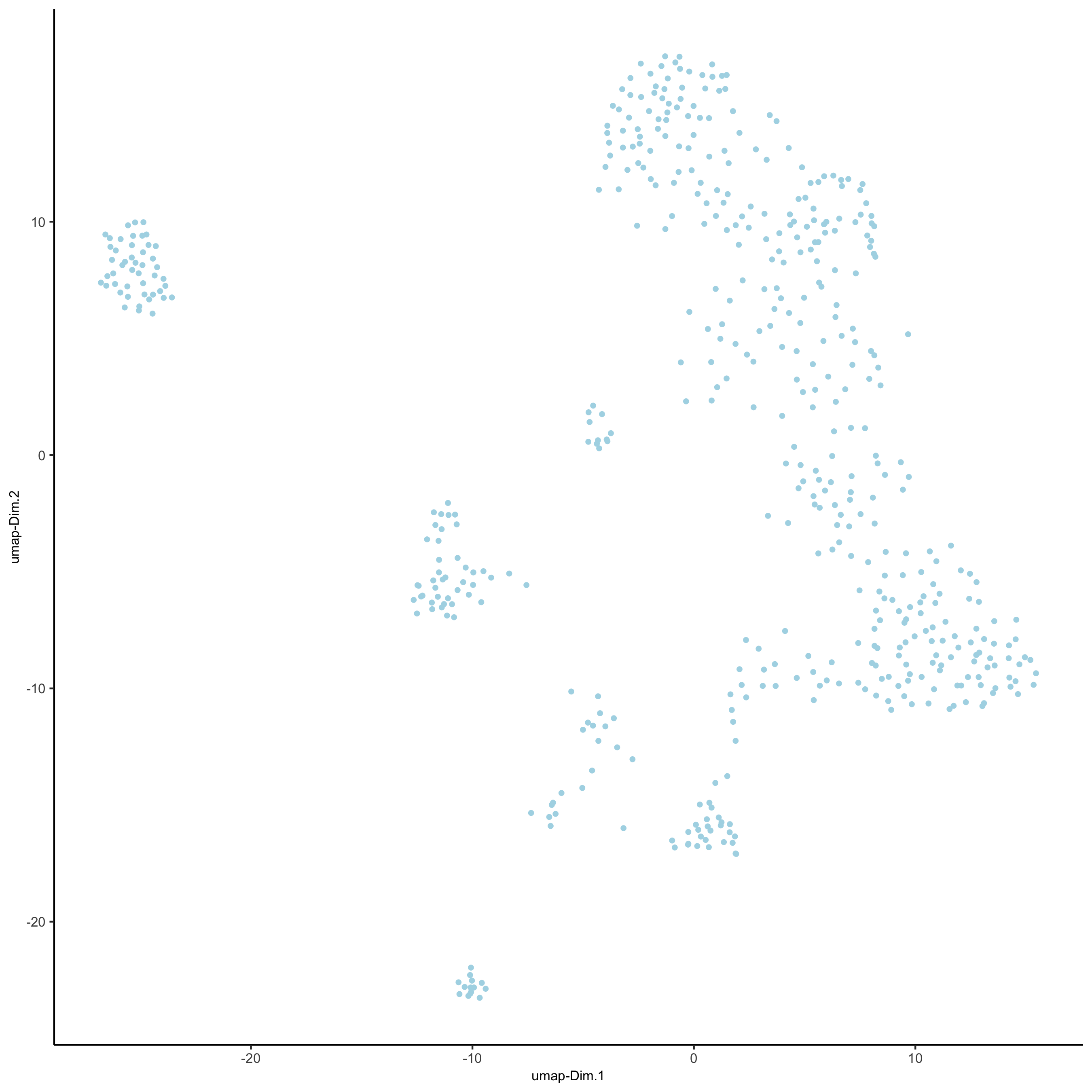
## run UMAP and tSNE on PCA space (default)
SS_seqfish <- runUMAP(SS_seqfish, dimensions_to_use = 1:15, n_threads = 10)
plotUMAP(gobject = SS_seqfish,save_param = list(save_name = '3_d_UMAP_reduction'))
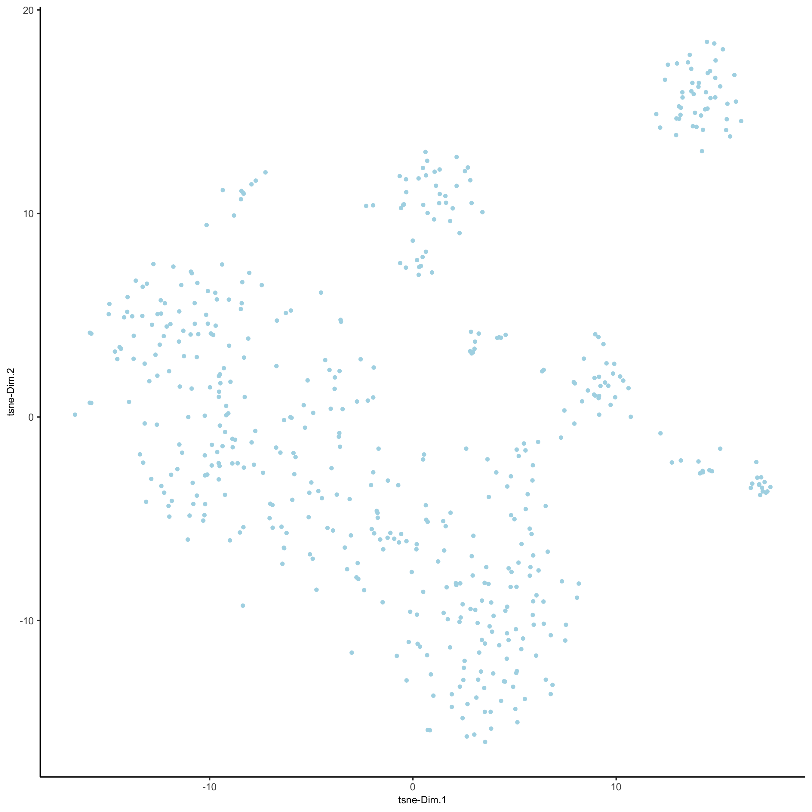
SS_seqfish <- runtSNE(SS_seqfish, dimensions_to_use = 1:15)
plotTSNE(gobject = SS_seqfish,save_param = list(save_name = '3_e_tSNE_reduction'))

3_b_screeplot.png

3_c_PCA_reduction.png

3_d_UMAP_reduction.png

3_e_tSNE_reduction.png

4. Nearest neighbor network and clustering

SS_seqfish <- createNearestNetwork(gobject = SS_seqfish, dimensions_to_use = 1:15, k = 15)

4.1. Leiden clustering

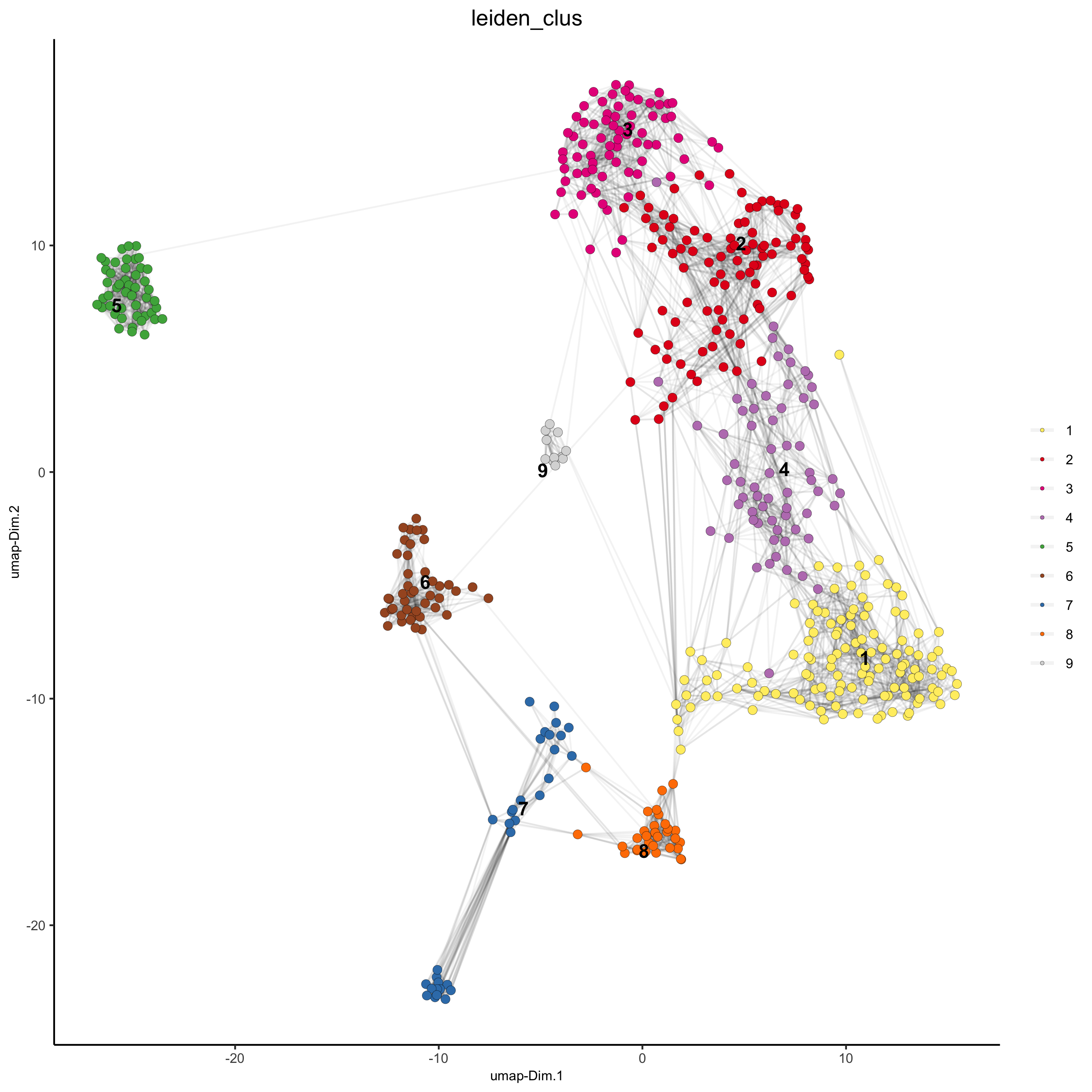
SS_seqfish <- doLeidenCluster(gobject = SS_seqfish, resolution = 0.4, n_iterations = 1000)
plotUMAP(gobject = SS_seqfish,cell_color = 'leiden_clus', show_NN_network = T, point_size = 2.5,save_param = list(save_name = '4_a_UMAP_leiden'))
## Leiden subclustering for specified clusters
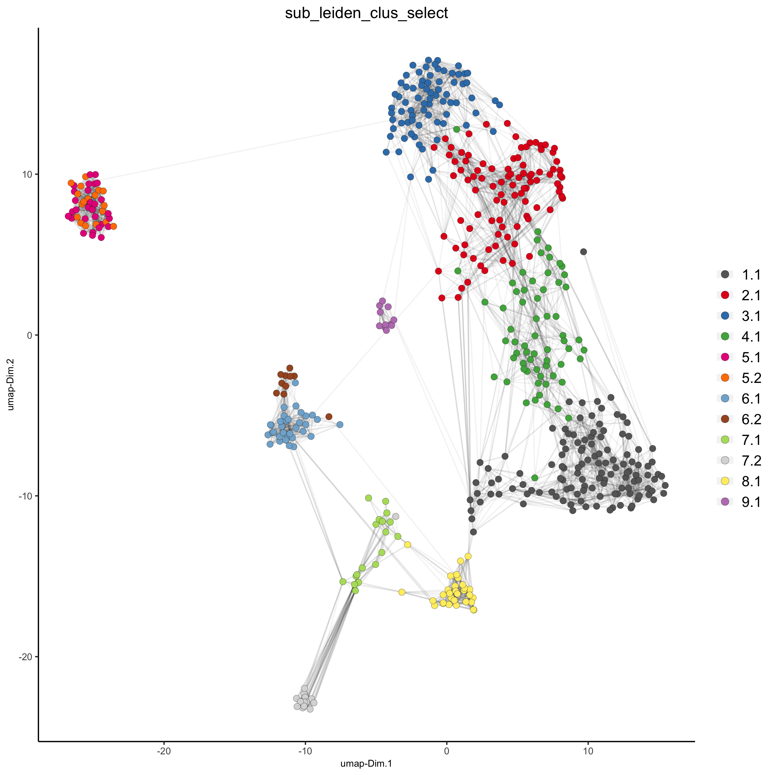
SS_seqfish = doLeidenSubCluster(gobject = SS_seqfish, cluster_column = 'leiden_clus',resolution = 0.2, k_neighbors = 10,hvg_param = list(method = 'cov_loess', difference_in_cov = 0.1),pca_param = list(expression_values = 'normalized', scale_unit = F),nn_param = list(dimensions_to_use = 1:5), selected_clusters = c(5, 6, 7),name = 'sub_leiden_clus_select')
## set colors for clusters
subleiden_order = c( 1.1, 5.1, 5.2,  2.1, 3.1,4.1,  4.2, 4.3, 6.2, 6.1,7.1, 7.2, 9.1, 8.1)
subleiden_colors = Giotto:::getDistinctColors(length(subleiden_order)) 
names(subleiden_colors) = subleiden_order
plotUMAP(gobject = SS_seqfish,cell_color = 'sub_leiden_clus_select', cell_color_code = subleiden_colors,show_NN_network = T, point_size = 2.5, show_center_label = F, legend_text = 12, legend_symbol_size = 3,save_param = list(save_name = '4_b_UMAP_leiden_subcluster'))

4_a_UMAP_leiden.png

4_b_UMAP_leiden_subcluster.png

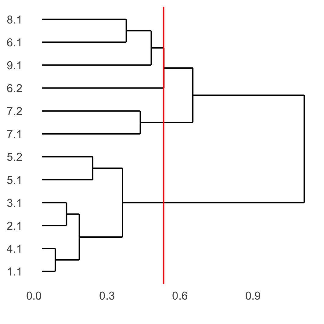
4.2. Cluster relationship

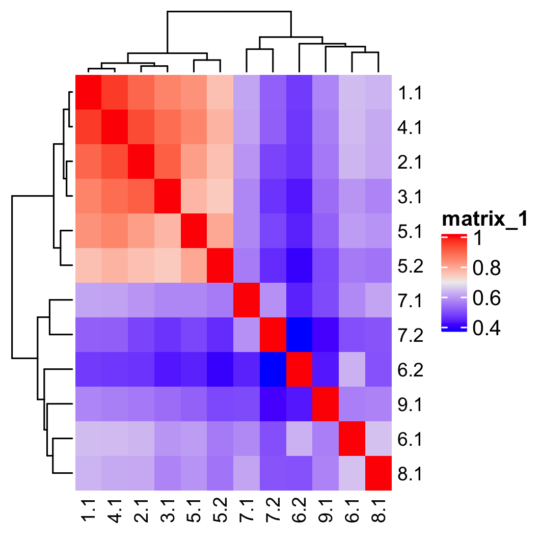
showClusterHeatmap(gobject = SS_seqfish, cluster_column = 'sub_leiden_clus_select',save_param = list(save_name = '4_c_heatmap', units = 'cm'),row_names_gp = grid::gpar(fontsize = 9), column_names_gp = grid::gpar(fontsize = 9))
showClusterDendrogram(SS_seqfish, h = 0.5, rotate = T, cluster_column = 'sub_leiden_clus_select', save_param = list(save_name = '4_d_dendro', units = 'cm'))

4_c_heatmap.png

4_d_dendro.png

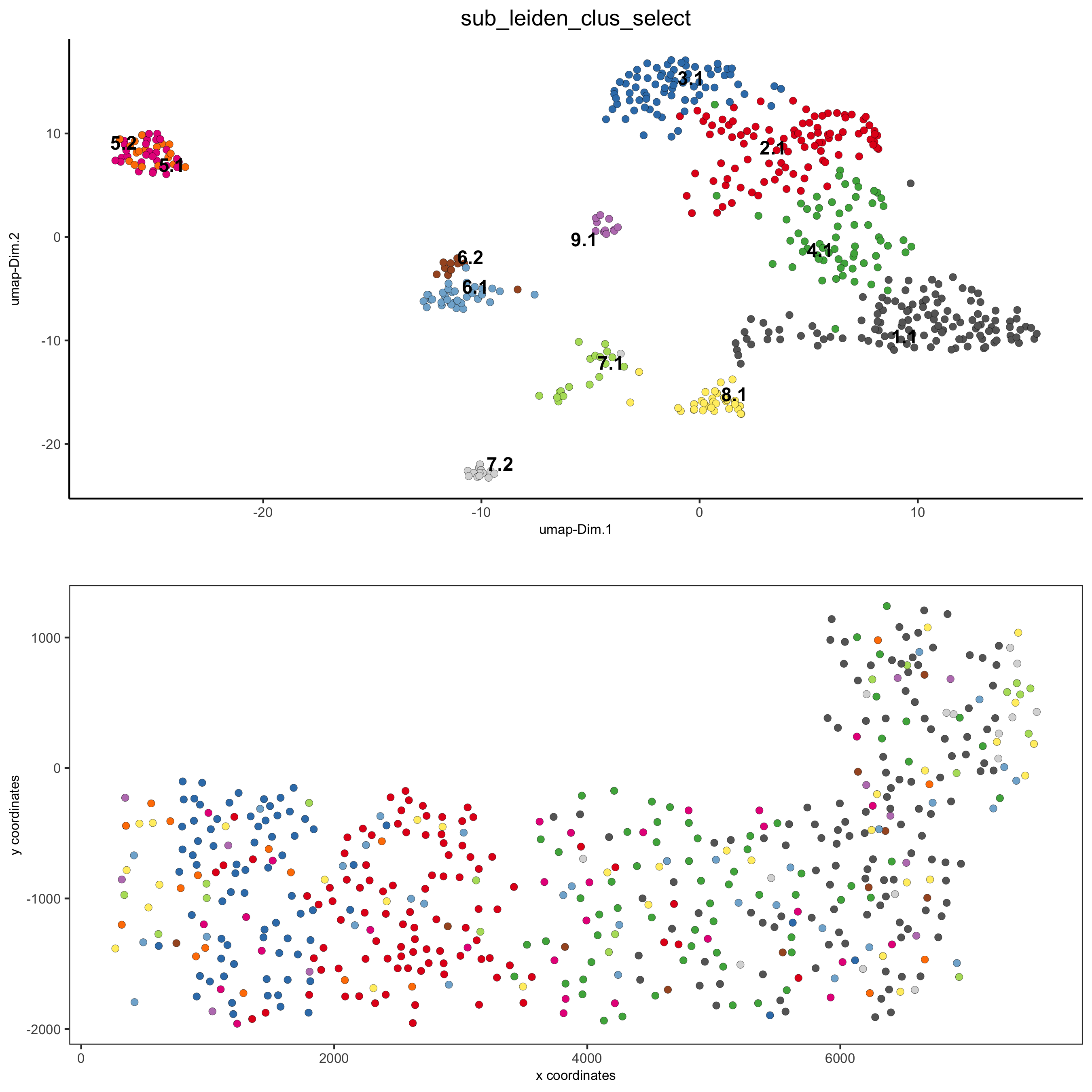
5. Visualize spatial and expression spaces

5.1. Expression and spatial

spatDimPlot(gobject = SS_seqfish, cell_color = 'sub_leiden_clus_select', cell_color_code = subleiden_colors, dim_point_size = 2, spat_point_size = 2,save_param = list(save_name = '5_a_covis_leiden'))
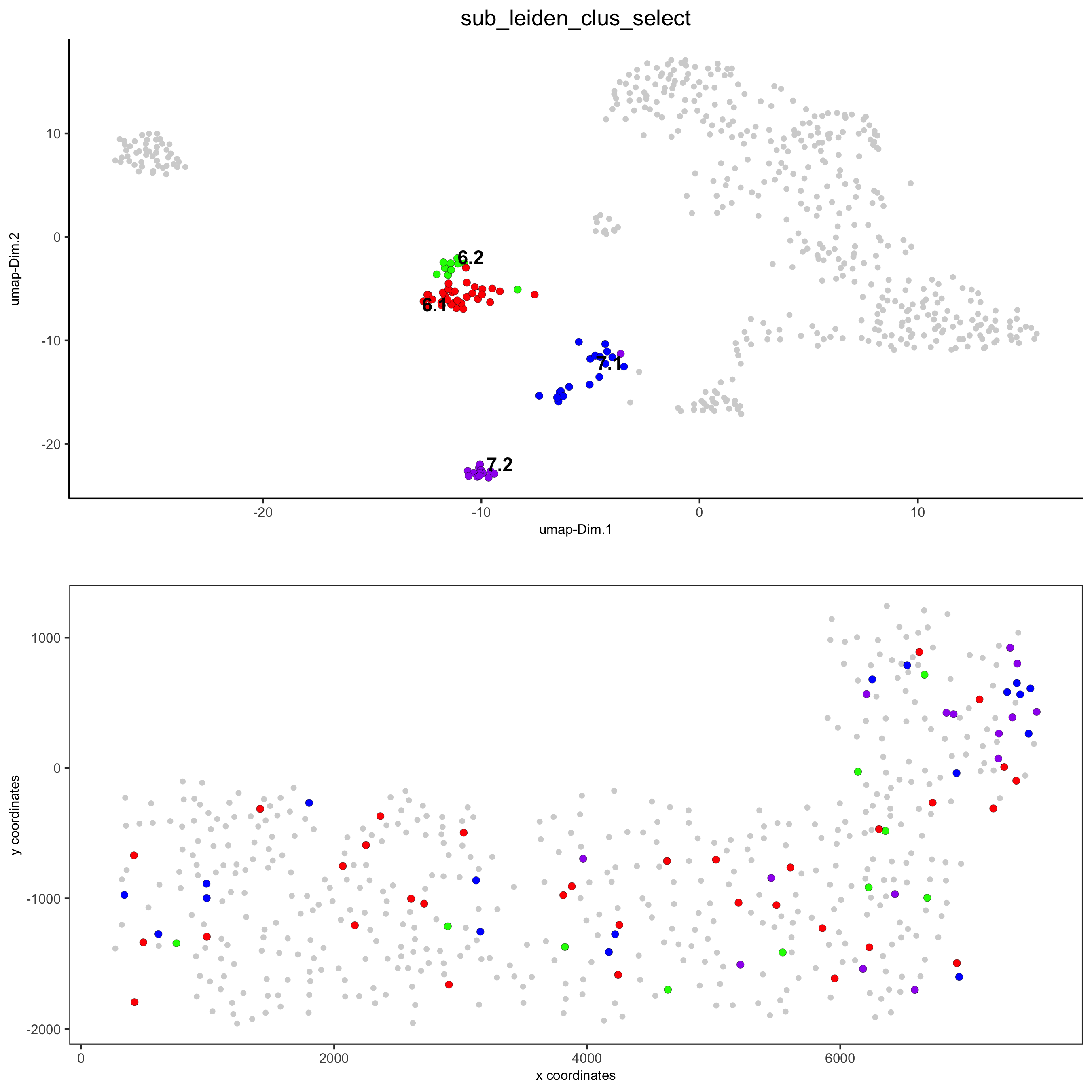
# selected groups and provide new colors
groups_of_interest = c(6.1, 6.2, 7.1, 7.2)
group_colors = c('red', 'green', 'blue', 'purple'); names(group_colors) = groups_of_interest
spatDimPlot(gobject = SS_seqfish, cell_color = 'sub_leiden_clus_select', dim_point_size = 2, spat_point_size = 2,select_cell_groups = groups_of_interest, cell_color_code = group_colors,save_param = list(save_name = '5_b_covis_leiden_selected'))

5_a_covis_leiden.png

5_b_covis_leiden_selected.png

6. Cell type marker gene detection

We illustrate the Gini method, though other methods such as scran is also available.

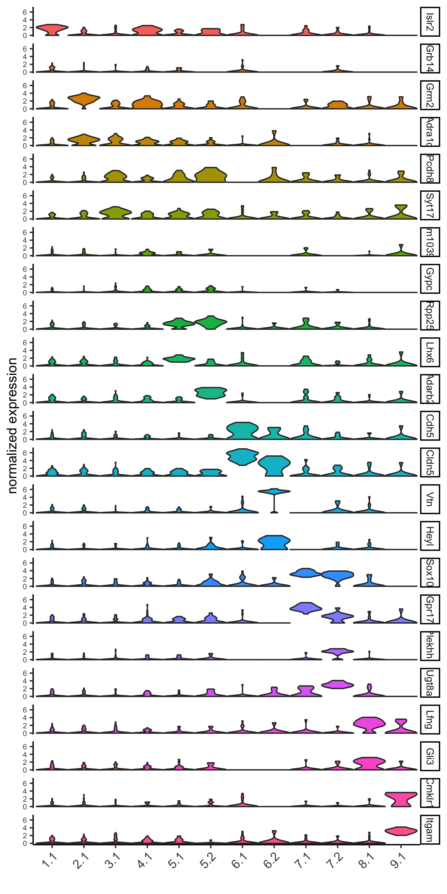
6.1. Gini

gini_markers_subclusters = findMarkers_one_vs_all(gobject = SS_seqfish,method = 'gini', expression_values = 'normalized',cluster_column = 'sub_leiden_clus_select', min_genes = 20, min_expr_gini_score = 0.5, min_det_gini_score = 0.5)
topgenes_gini = gini_markers_subclusters[, head(.SD, 2), by = 'cluster']
# violinplot
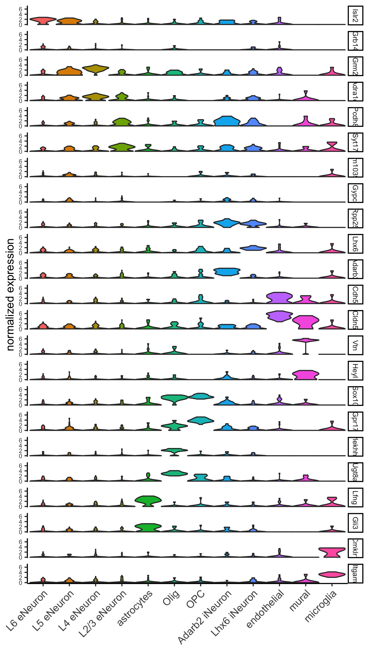
violinPlot(SS_seqfish, genes = unique(topgenes_gini$genes), cluster_column = 'sub_leiden_clus_select',strip_text = 8, strip_position = 'right', cluster_custom_order = unique(topgenes_gini$cluster),save_param = c(save_name = '6_a_violinplot_gini', base_width = 5, base_height = 10))
# cluster heatmap
topgenes_gini2 = gini_markers_subclusters[, head(.SD, 6), by = 'cluster']
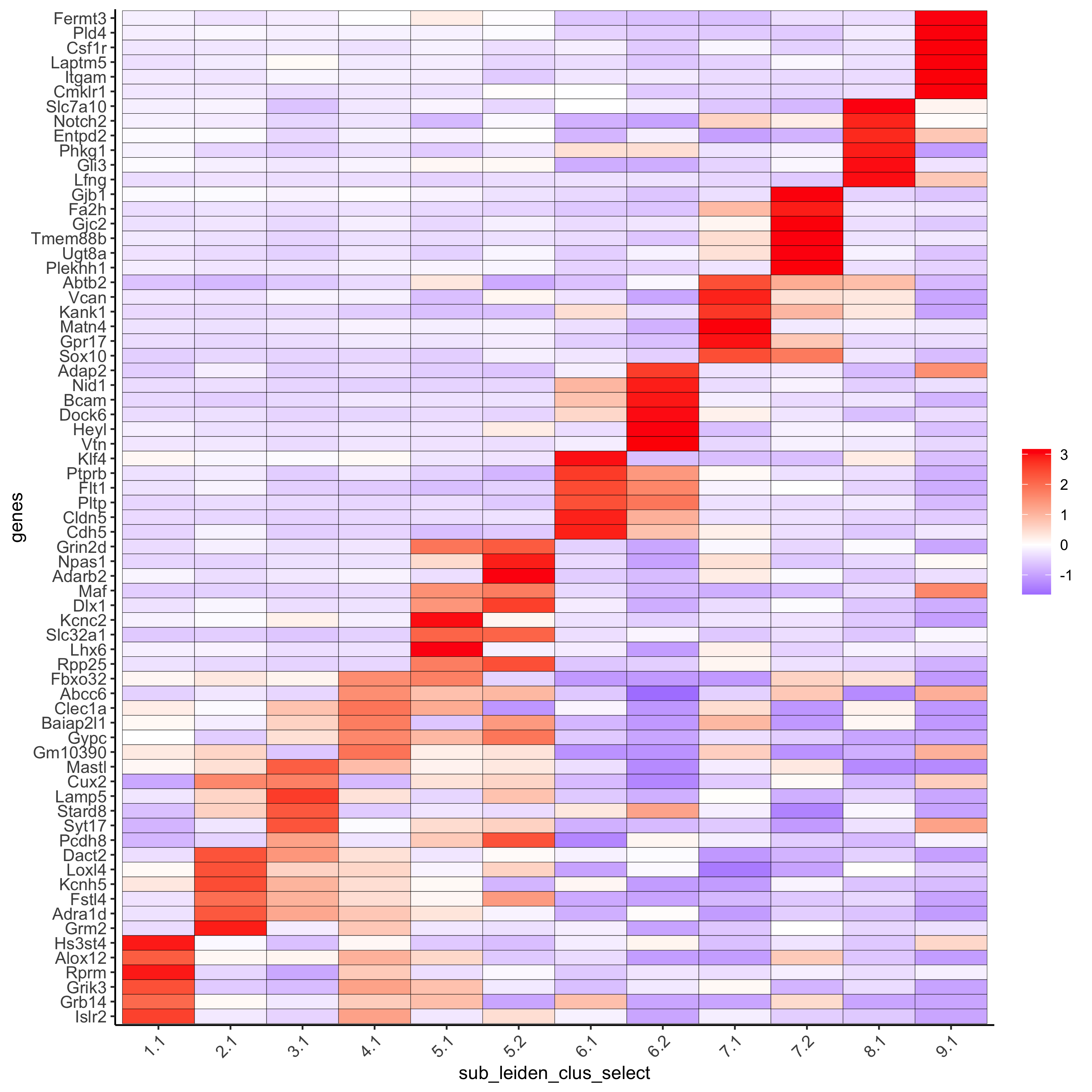
plotMetaDataHeatmap(SS_seqfish, selected_genes = unique(topgenes_gini2$genes), custom_gene_order = unique(topgenes_gini2$genes),custom_cluster_order = unique(topgenes_gini2$cluster),metadata_cols = c('sub_leiden_clus_select'), x_text_size = 10, y_text_size = 10,save_param = c(save_name = '6_b_metaheatmap_gini'))

6_a_violinplot_gini.png

6_b_metaheatmap_gini.png

7. Cell type annotation

7.1. General cell types

#create vector with names
clusters_cell_types_cortex = c('L6 eNeuron', 'L4 eNeuron', 'L2/3 eNeuron', 'L5 eNeuron', 'Lhx6 iNeuron', 'Adarb2 iNeuron', 'endothelial', 'mural','OPC','Olig','astrocytes', 'microglia')
names(clusters_cell_types_cortex) = c(1.1, 2.1, 3.1, 4.1,5.1, 5.2,6.1, 6.2, 7.1, 7.2,8.1, 9.1)
SS_seqfish = annotateGiotto(gobject = SS_seqfish, annotation_vector = clusters_cell_types_cortex,
cluster_column = 'sub_leiden_clus_select', name = 'cell_types')
# cell type order and colors
cell_type_order = c('L6 eNeuron', 'L5 eNeuron', 'L4 eNeuron', 'L2/3 eNeuron','astrocytes', 'Olig', 'OPC','Adarb2 iNeuron', 'Lhx6 iNeuron','endothelial', 'mural', 'microglia')
cell_type_colors = subleiden_colors
names(cell_type_colors) = clusters_cell_types_cortex[names(subleiden_colors)]
cell_type_colors = cell_type_colors[cell_type_order]
## violinplot
violinPlot(gobject = SS_seqfish, genes = unique(topgenes_gini$genes),strip_text = 7, strip_position = 'right', cluster_custom_order = cell_type_order,cluster_column = 'cell_types', color_violin = 'cluster',save_param = c(save_name = '7_a_violinplot', base_width = 5))
## co-visualization
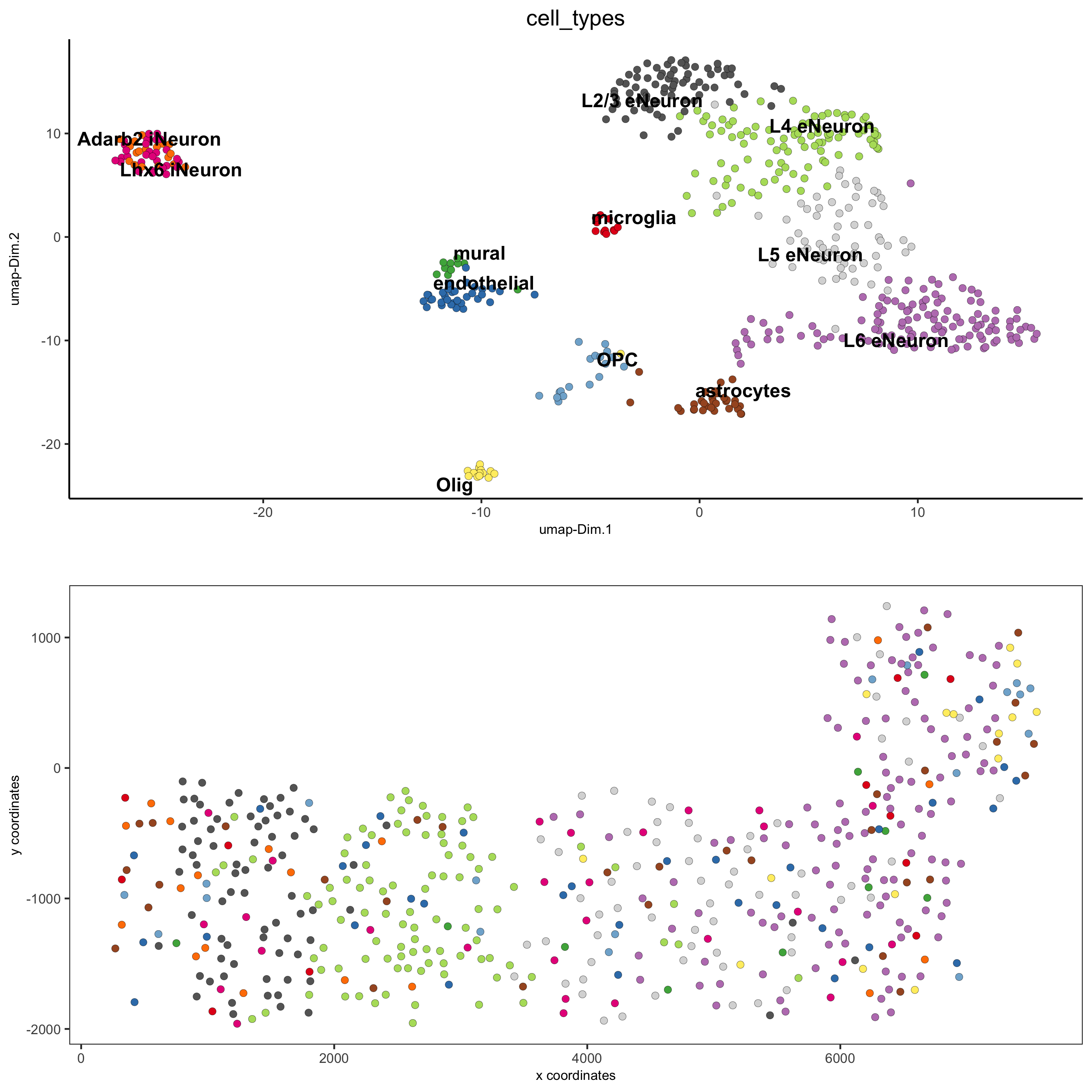
spatDimPlot(gobject = SS_seqfish, cell_color = 'cell_types',dim_point_size = 2, spat_point_size = 2, dim_show_cluster_center = F, dim_show_center_label = T,save_param = c(save_name = '7_b_covisualization'))

7_a_violinplot.png

7_b_covisualization.png

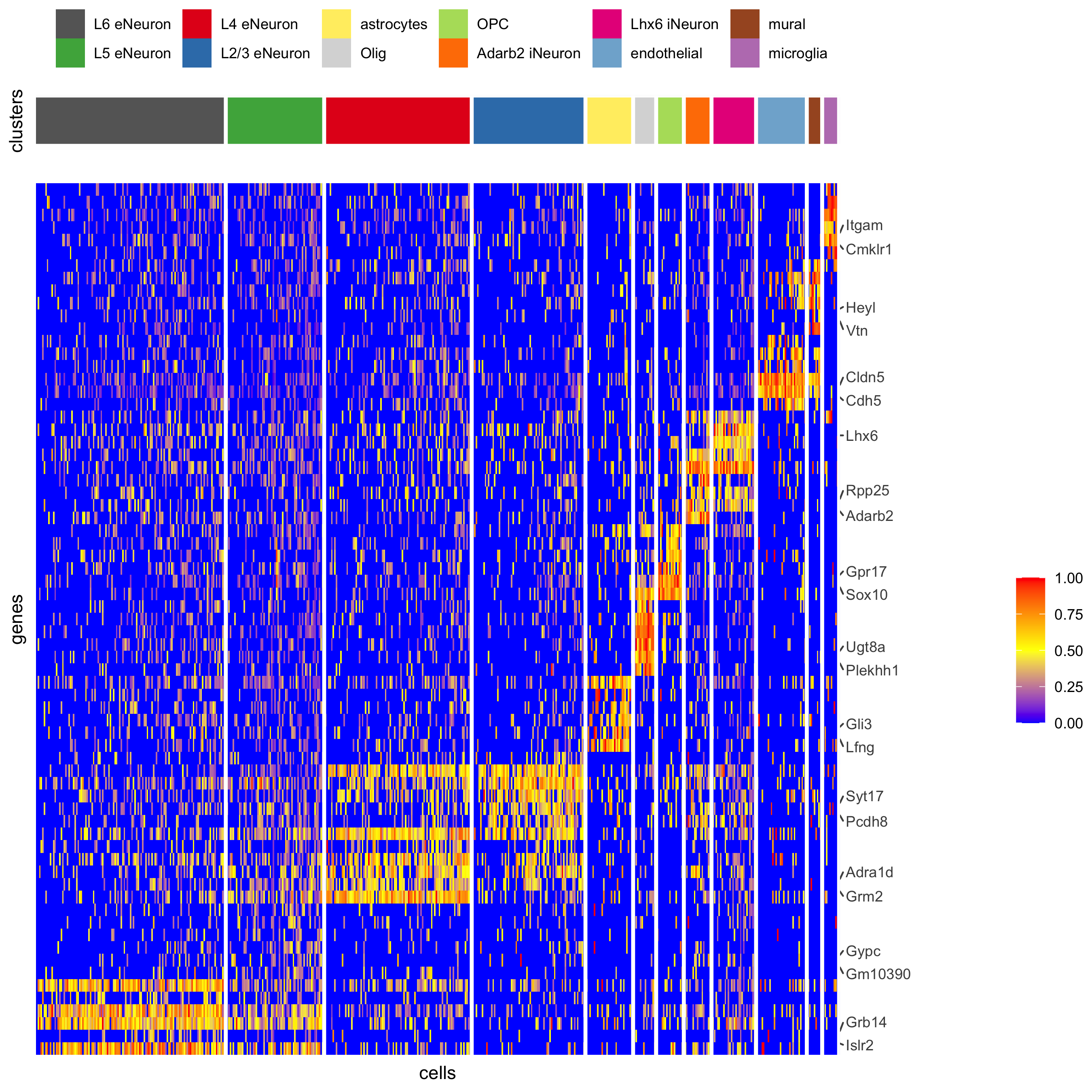
## heatmap genes vs cells
gini_markers_subclusters[, cell_types := clusters_cell_types_cortex[cluster] ]
gini_markers_subclusters[, cell_types := factor(cell_types, cell_type_order)]
data.table::setorder(gini_markers_subclusters, cell_types)
plotHeatmap(gobject = SS_seqfish,genes = gini_markers_subclusters[, head(.SD, 3), by = 'cell_types']$genes, gene_order = 'custom',gene_custom_order = unique(gini_markers_subclusters[, head(.SD, 3), by = 'cluster']$genes),cluster_column = 'cell_types', cluster_order = 'custom',cluster_custom_order = unique(gini_markers_subclusters[, head(.SD, 3), by = 'cell_types']$cell_types), legend_nrows = 2,save_param = c(save_name = '7_c_heatmap'))
plotHeatmap(gobject = SS_seqfish,cluster_color_code = cell_type_colors,genes = gini_markers_subclusters[, head(.SD, 6), by = 'cell_types']$genes,gene_order = 'custom',gene_label_selection = gini_markers_subclusters[, head(.SD, 2), by = 'cluster']$genes,gene_custom_order = unique(gini_markers_subclusters[, head(.SD, 6), by = 'cluster']$genes),cluster_column = 'cell_types', cluster_order = 'custom',cluster_custom_order = unique(gini_markers_subclusters[, head(.SD, 3), by = 'cell_types']$cell_types), legend_nrows = 2,save_param = c(save_name = '7_d_heatmap_selected'))

7_c_heatmap.png

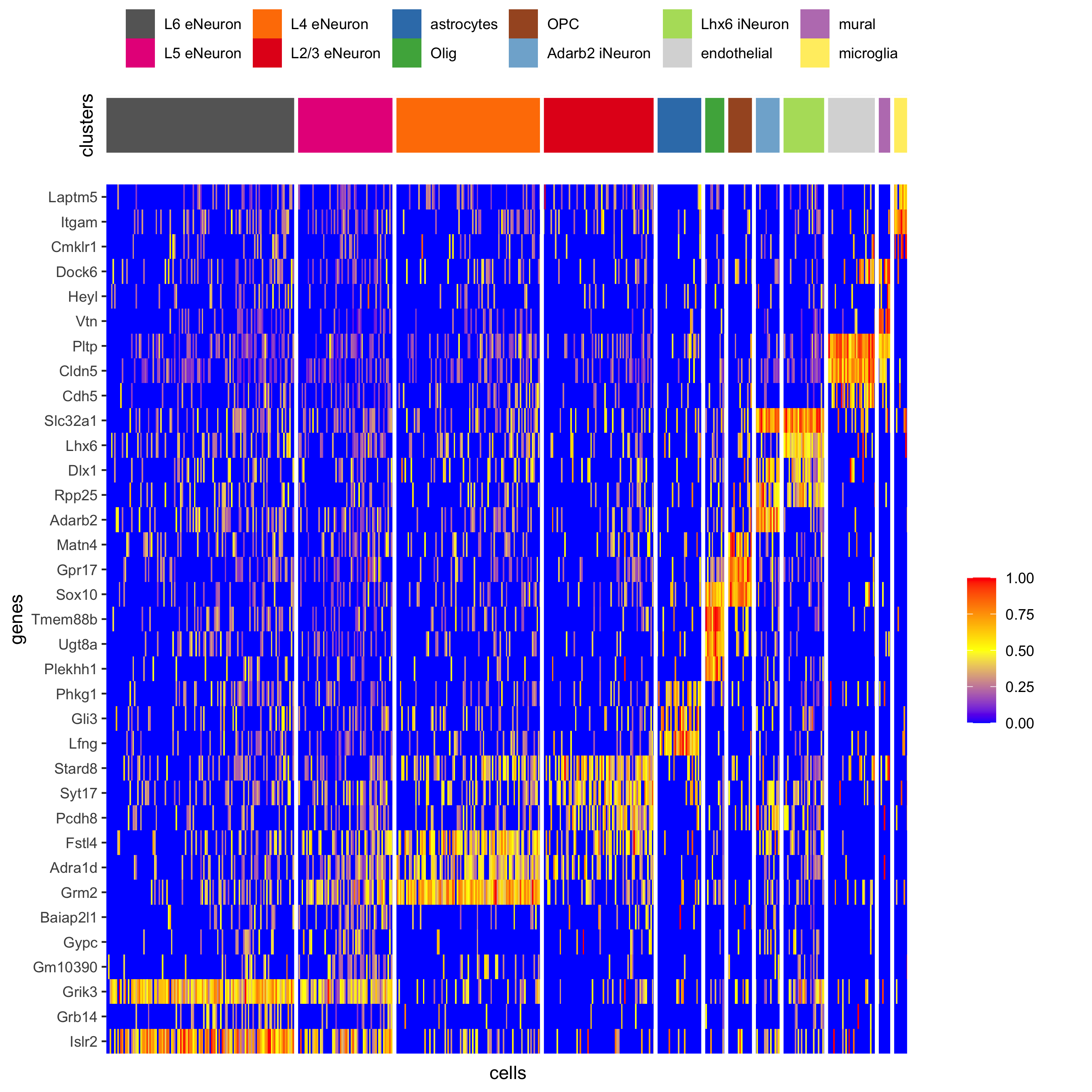
7_d_heatmap_selected.png

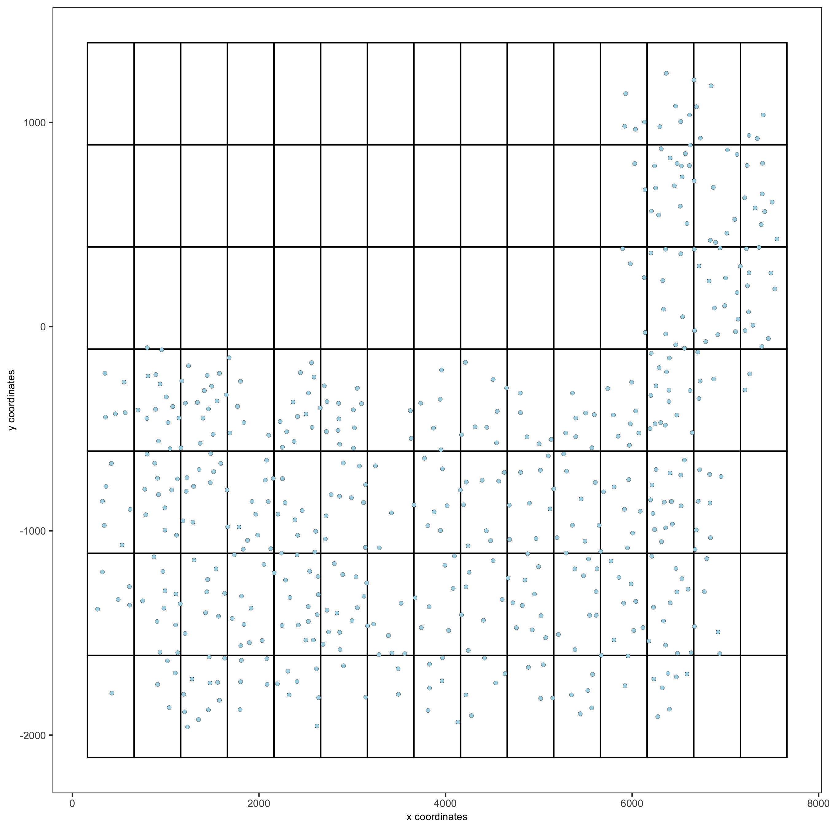
8. Spatial grid

SS_seqfish <- createSpatialGrid(gobject = SS_seqfish,sdimx_stepsize = 500,sdimy_stepsize = 500,minimum_padding = 50)
spatPlot(gobject = SS_seqfish, show_grid = T, point_size = 1.5,save_param = c(save_name = '8_a_grid'))

8_a_grid.png

9. Spatial network

9.1. delaunay network: stats + creation

plotStatDelaunayNetwork(gobject = SS_seqfish, maximum_distance = 400, save_plot = F)
SS_seqfish = createSpatialNetwork(gobject = SS_seqfish, minimum_k = 2, maximum_distance_delaunay = 400)

9.2. Create spatial networks based on k and/or distance from centroid

SS_seqfish <- createSpatialNetwork(gobject = SS_seqfish, method = 'kNN', k = 5, name = 'spatial_network')
SS_seqfish <- createSpatialNetwork(gobject = SS_seqfish, method = 'kNN', k = 10, name = 'large_network')
SS_seqfish <- createSpatialNetwork(gobject = SS_seqfish, method = 'kNN', k = 100,
maximum_distance_knn = 200, minimum_k = 2, name = 'distance_network')

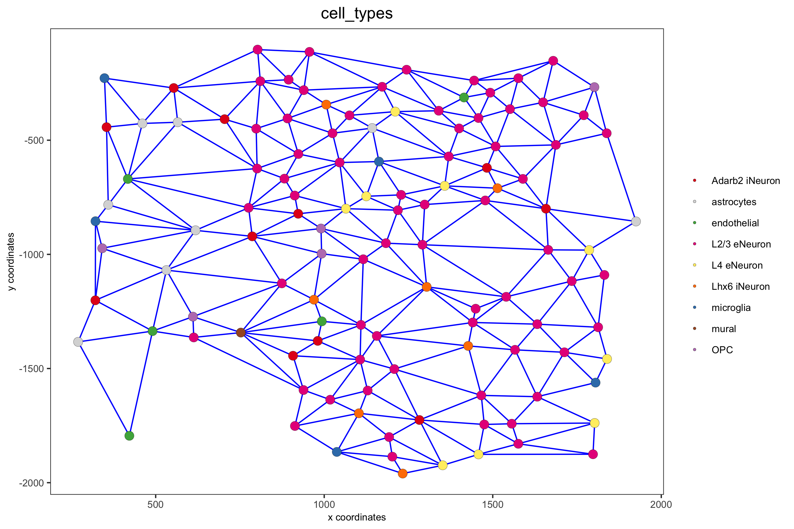
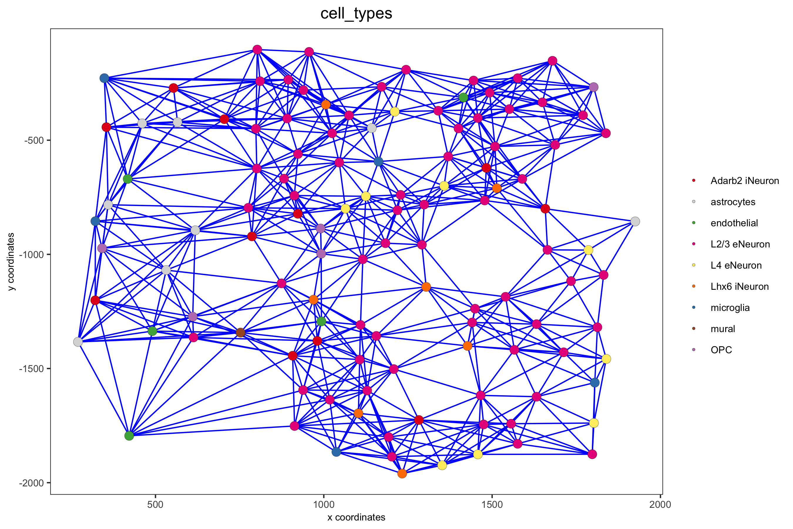
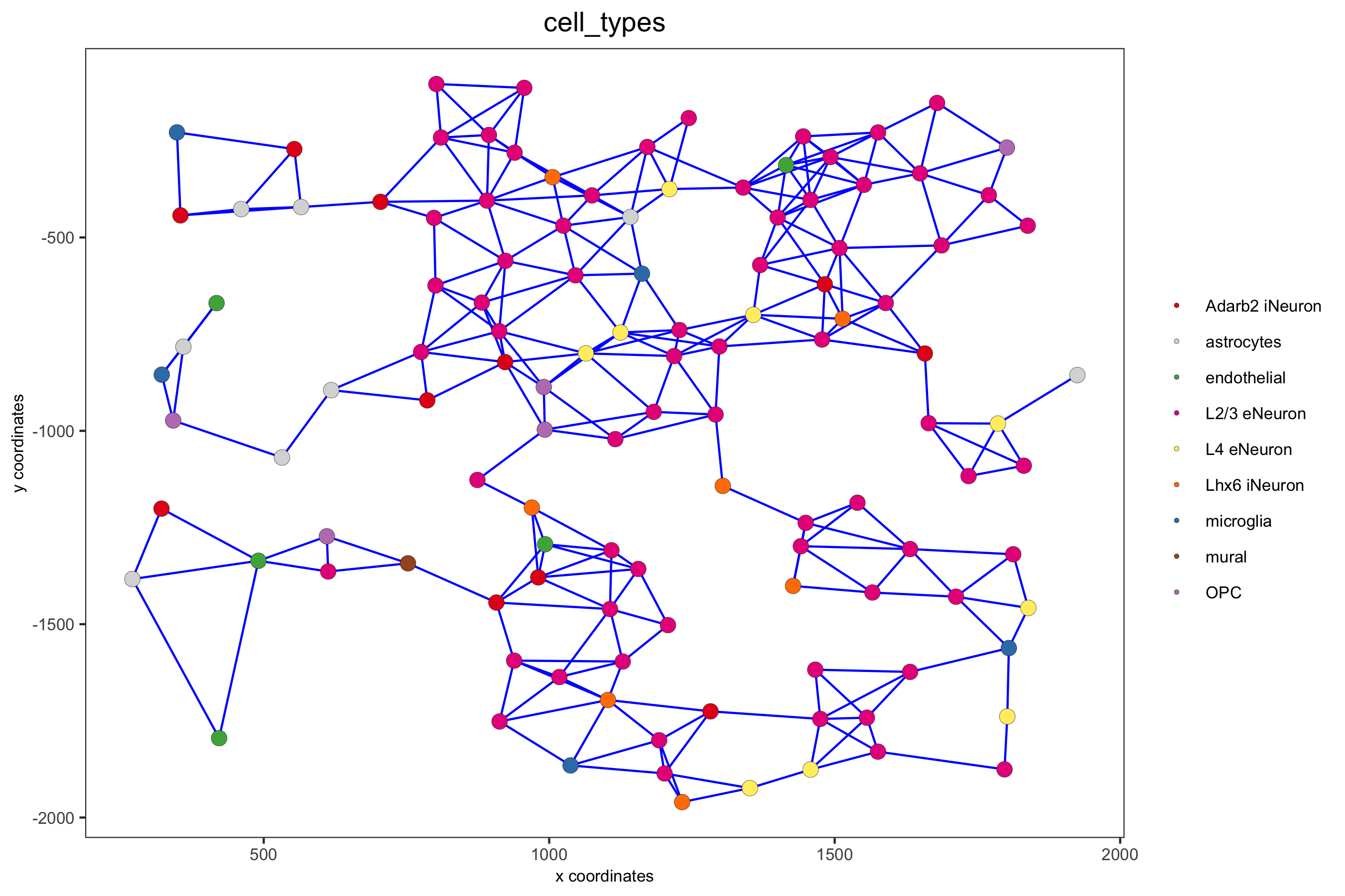
Visualize different spatial networks on first field (~ layer 1)

cell_metadata = pDataDT(SS_seqfish)
field1_ids = cell_metadata[FOV == 0]$cell_ID
subSS_seqfish = subsetGiotto(SS_seqfish, cell_ids = field1_ids)
spatPlot(gobject = subSS_seqfish, show_network = T,network_color = 'blue', spatial_network_name = 'Delaunay_network',point_size = 2.5, cell_color = 'cell_types', save_param = c(save_name = '9_a_spatial_network_delaunay', base_height = 6))
spatPlot(gobject = subSS_seqfish, show_network = T,network_color = 'blue', spatial_network_name = 'spatial_network',point_size = 2.5, cell_color = 'cell_types',save_param = c(save_name = '9_b_spatial_network_k3', base_height = 6))
spatPlot(gobject = subSS_seqfish, show_network = T,network_color = 'blue', spatial_network_name = 'large_network',point_size = 2.5, cell_color = 'cell_types',save_param = c(save_name = '9_c_spatial_network_k10', base_height = 6))
spatPlot(gobject = subSS_seqfish, show_network = T,network_color = 'blue', spatial_network_name = 'distance_network',point_size = 2.5, cell_color = 'cell_types',save_param = c(save_name = '9_d_spatial_network_dist', base_height = 6))

9_a_spatial_network_delaunay.png

9_b_spatial_network_k3.png

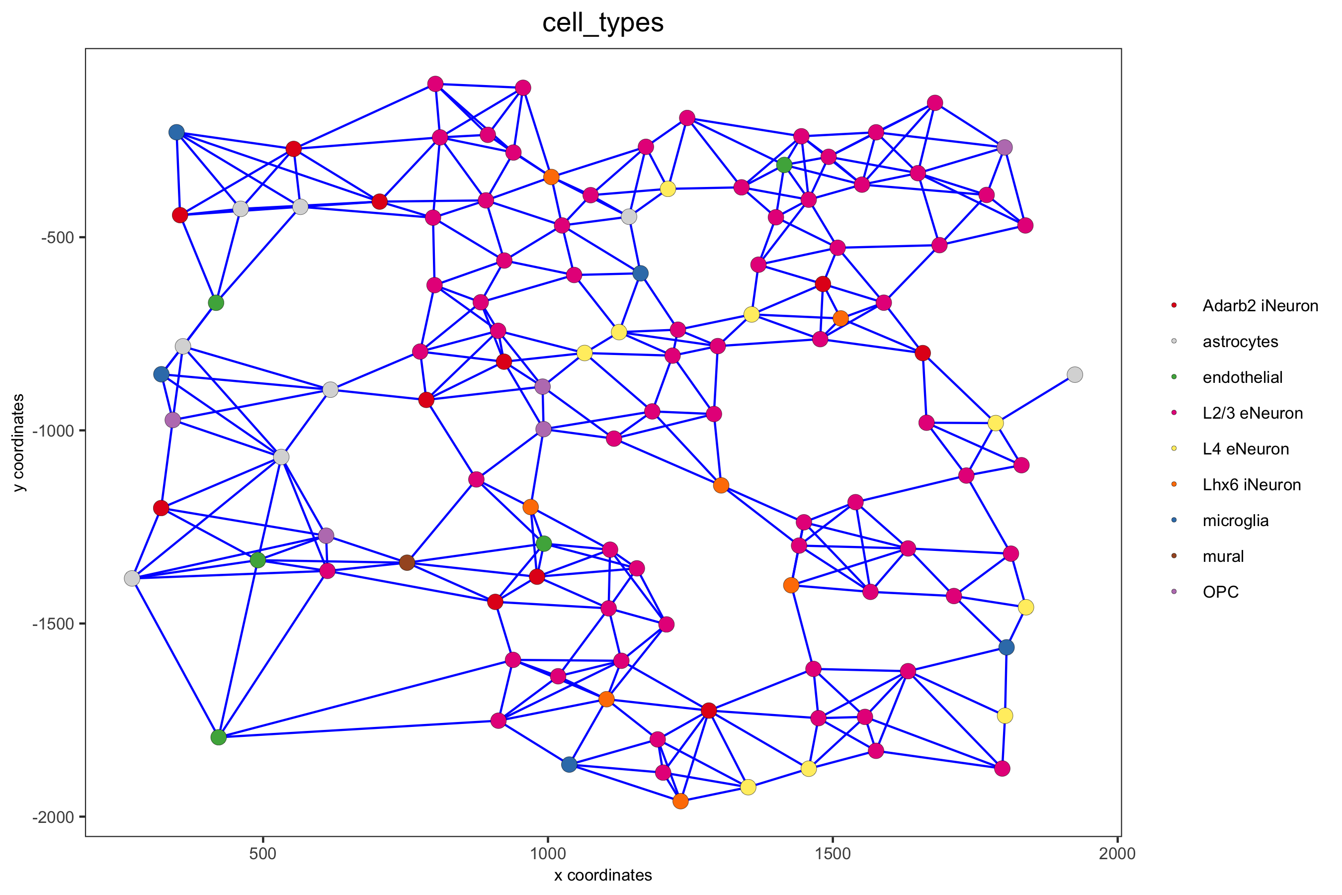
9_c_spatial_network_k10.png

9_d_spatial_network_dist.png

10. Spatial genes

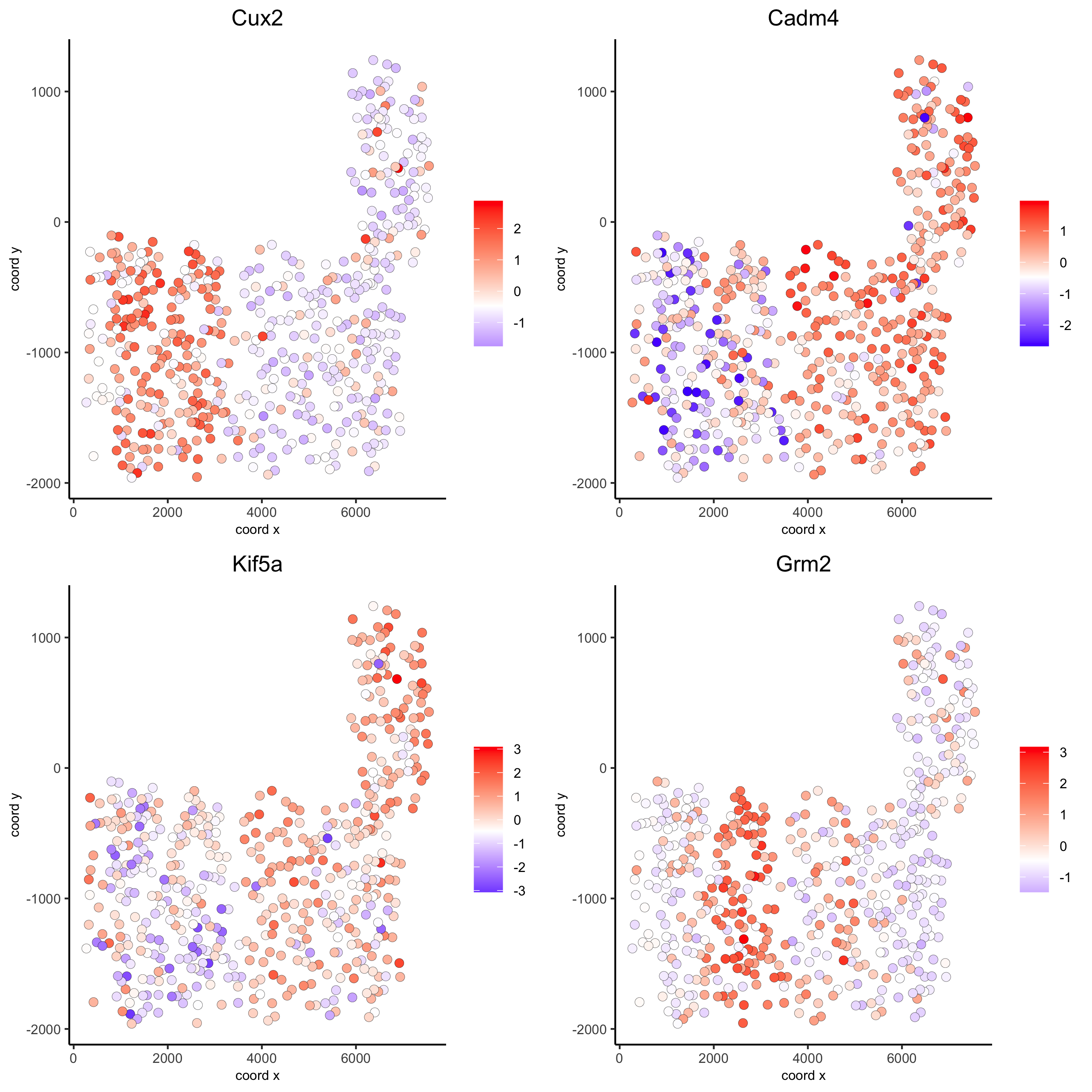
10.1. Individual spatial genes

We have a number of different ways to find spatial genes, including silhouetteRank, binSpect (kmeans and rank), developed by us, and SPARK, spatialDE, and trendceek, for which we created wrapers. We illustate the binSpect below.

km_spatialgenes = binSpect(SS_seqfish)
spatGenePlot(SS_seqfish, expression_values = 'scaled', genes = km_spatialgenes[1:4]$genes,point_shape = 'border', point_border_stroke = 0.1,show_network = F, network_color = 'lightgrey', point_size = 2.5, cow_n_col = 2,save_param = list(save_name = '10_a_spatialgenes_km'))

10_a_spatialgenes_km.png

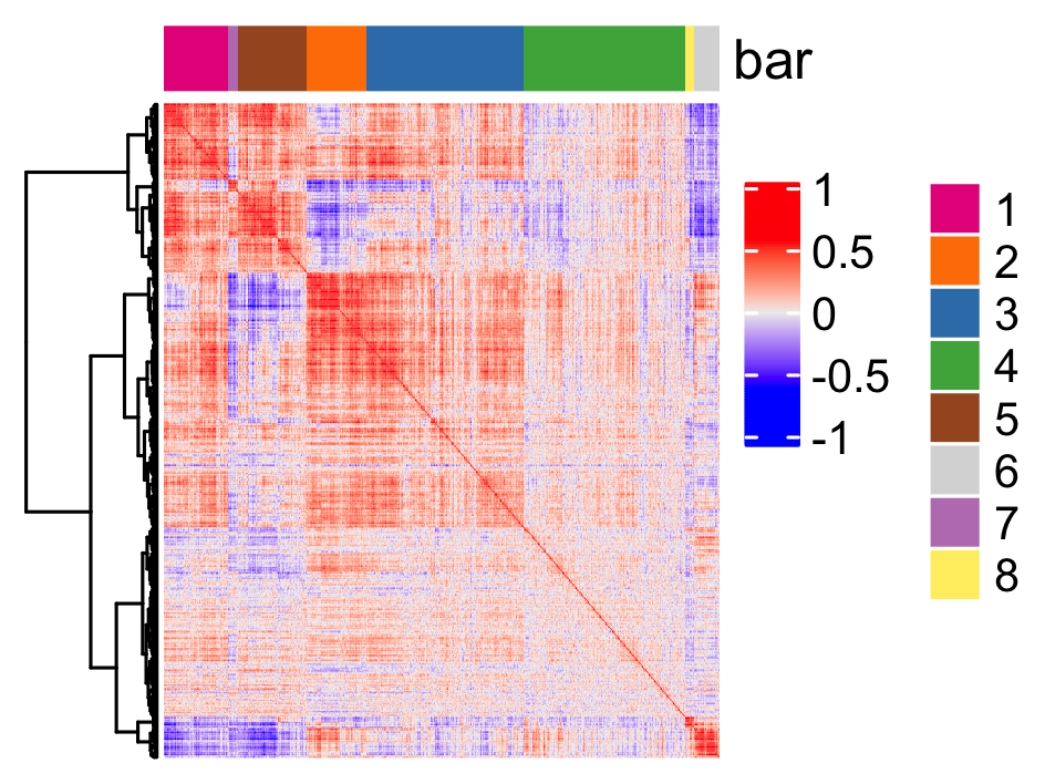
10.2. Spatial genes co-expression modules

ext_spatial_genes = km_spatialgenes[1:500]$genes

There are 4 steps:

1. calculate gene spatial correlation and single-cell correlation
2. cluster correlated genes & visualize
3. rank spatial correlated clusters and show genes for selected clusters
4. create metagene enrichment score for clusters

spat_cor_netw_DT = detectSpatialCorGenes(SS_seqfish, method = 'network', spatial_network_name = 'Delaunay_network',subset_genes = ext_spatial_genes)
spat_cor_netw_DT = clusterSpatialCorGenes(spat_cor_netw_DT, name = 'spat_netw_clus', k = 8)
heatmSpatialCorGenes(SS_seqfish, spatCorObject = spat_cor_netw_DT, use_clus_name = 'spat_netw_clus',save_param = c(save_name = '10_b_spatialcoexpression_heatmap',base_height = 6, base_width = 8, units = 'cm'), heatmap_legend_param = list(title = NULL))
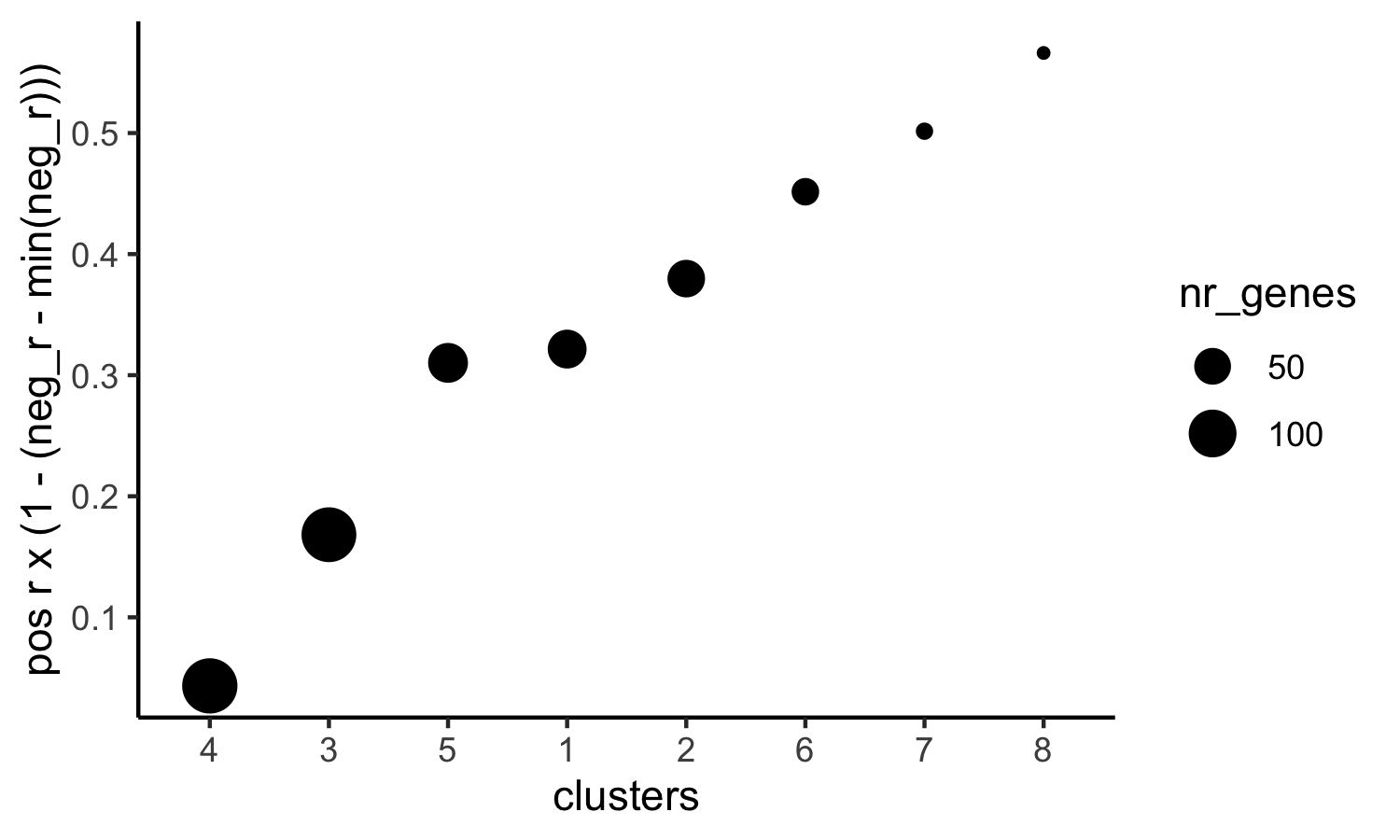
netw_ranks = rankSpatialCorGroups(SS_seqfish, spatCorObject = spat_cor_netw_DT, use_clus_name = 'spat_netw_clus',save_param = c(save_name = '10_c_spatialcoexpression_rank',base_height = 3, base_width = 5))
top_netw_spat_cluster = showSpatialCorGenes(spat_cor_netw_DT, use_clus_name = 'spat_netw_clus',selected_clusters = 6, show_top_genes = 1)
cluster_genes_DT = showSpatialCorGenes(spat_cor_netw_DT, use_clus_name = 'spat_netw_clus', show_top_genes = 1)
cluster_genes = cluster_genes_DT$clus; names(cluster_genes) = cluster_genes_DT$gene_ID
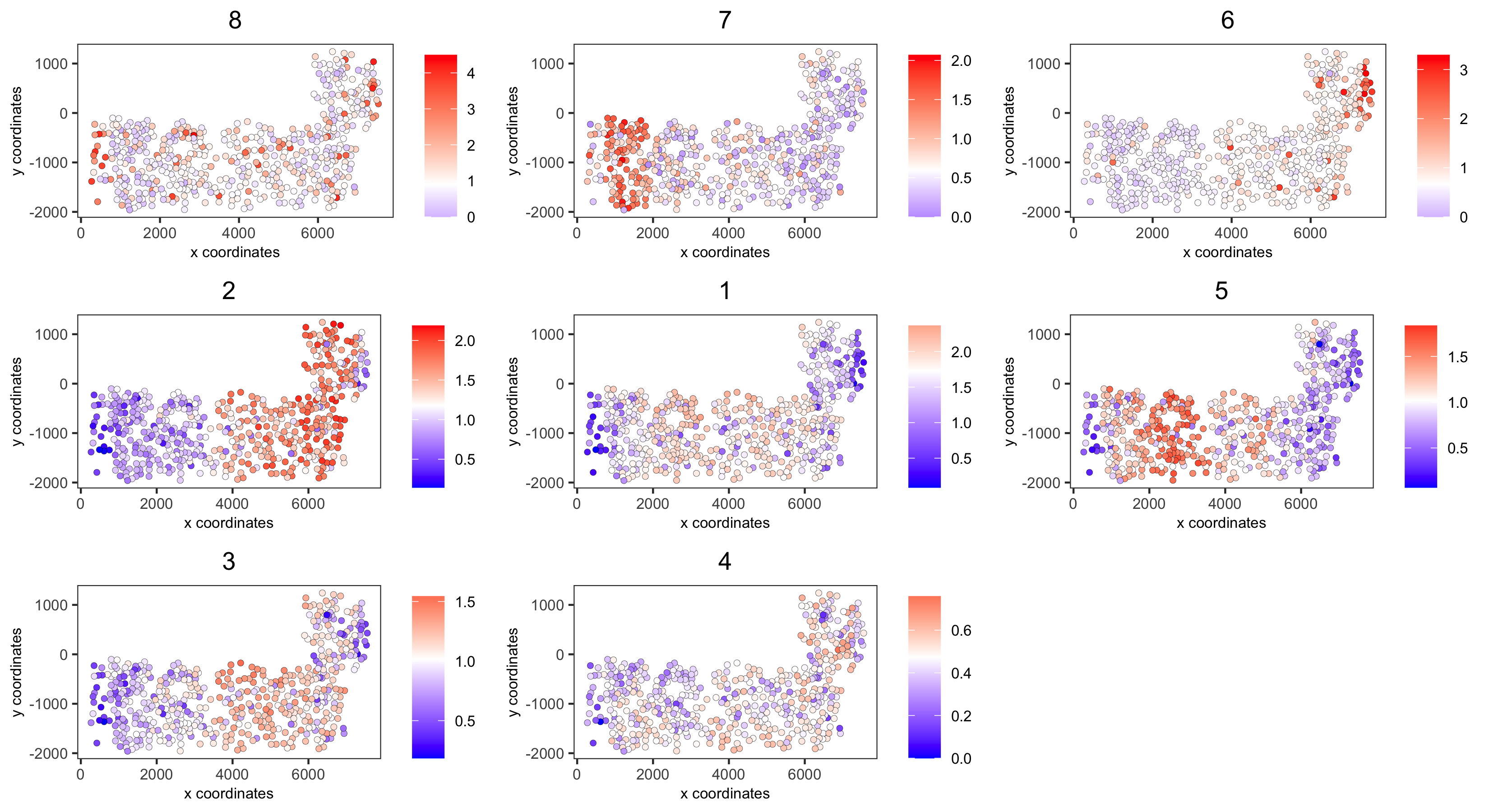
SS_seqfish = createMetagenes(SS_seqfish, gene_clusters = cluster_genes, name = 'cluster_metagene')
spatCellPlot(SS_seqfish,spat_enr_names = 'cluster_metagene',cell_annotation_values = netw_ranks$clusters,point_size = 1.5, cow_n_col = 3,save_param = c(save_name = '10_d_spatialcoexpression_metagenes',base_width = 11, base_height = 6))

10_b_spatialcoexpression_heatmap.png

10_c_spatialcoexpression_rank.png

10_d_spatialcoexpression_metagenes.png

11. HMRF spatial domains

hmrf_folder = fs::path(my_working_dir,'11_HMRF/')
if(!file.exists(hmrf_folder)) dir.create(hmrf_folder, recursive = T)
my_spatial_genes = km_spatialgenes[1:100]$genes
# do HMRF with different betas
HMRF_spatial_genes = doHMRF(gobject = SS_seqfish, expression_values = 'scaled',spatial_genes = my_spatial_genes,spatial_network_name = 'Delaunay_network',k = 9,betas = c(28,2,3), output_folder = paste0(hmrf_folder, '/', 'Spatial_genes/SG_top100_k9_scaled'))
## view results of HMRF
for(i in seq(28, 32, by = 2)) {
viewHMRFresults2D(gobject = SS_seqfish,HMRFoutput = HMRF_spatial_genes,k = 9, betas_to_view = i,point_size = 2)
}
## add HMRF of interest to giotto object
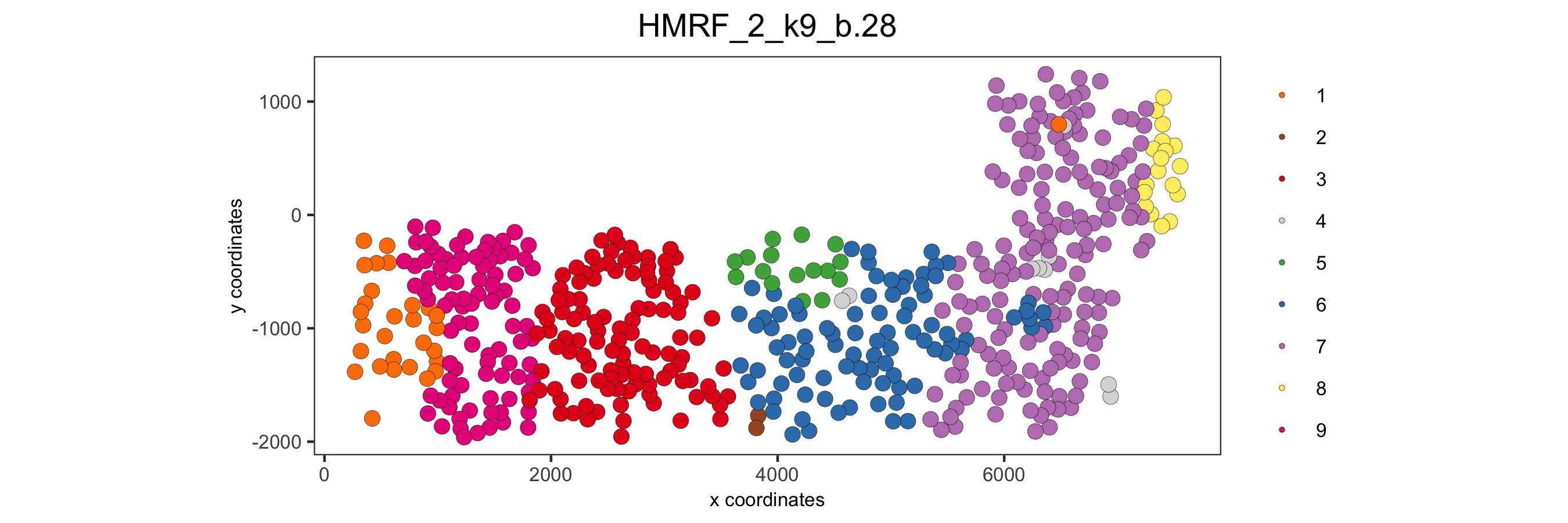
SS_seqfish = addHMRF(gobject = SS_seqfish,HMRFoutput = HMRF_spatial_genes,k = 9, betas_to_add = c(28),hmrf_name = 'HMRF_2')
## visualize
spatPlot(gobject = SS_seqfish, cell_color = 'HMRF_2_k9_b.28', point_size = 3, coord_fix_ratio = 1, save_param = c(save_name = '11_HMRF_2_k9_b.28', base_height = 3, base_width = 9, save_format = 'png'))

11_HMRF_2_k9_b.28.png

12. Cell neighborhood

12.1. cell-type/cell-type interactions

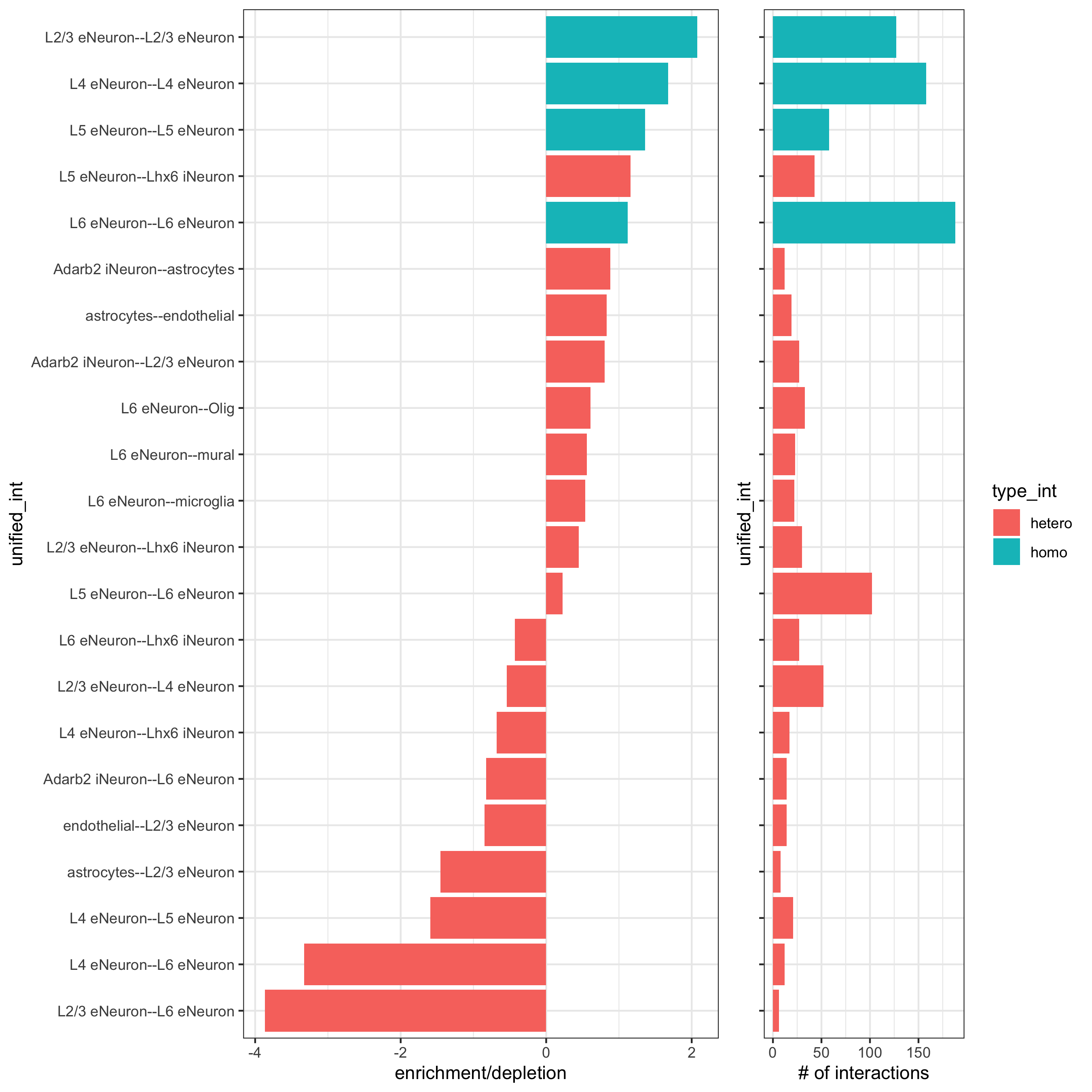
cell_proximities = cellProximityEnrichment(gobject = SS_seqfish,cluster_column = 'cell_types',spatial_network_name = 'Delaunay_network',adjust_method = 'fdr',number_of_simulations = 2000)
## barplot
cellProximityBarplot(gobject = SS_seqfish,CPscore = cell_proximities, min_orig_ints = 5, min_sim_ints = 5, save_param = c(save_name = '12_a_barplot_cell_cell_enrichment'))
## heatmap
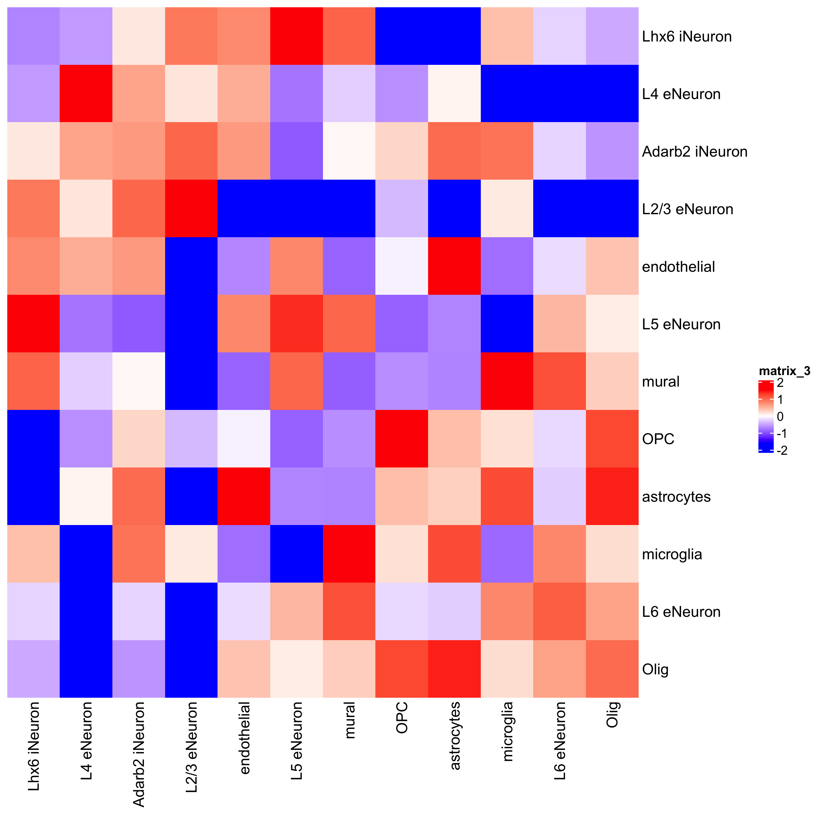
cellProximityHeatmap(gobject = SS_seqfish, CPscore = cell_proximities, order_cell_types = T, scale = T,color_breaks = c(-1.5, 0, 1.5), color_names = c('blue', 'white', 'red'),save_param = c(save_name = '12_b_heatmap_cell_cell_enrichment', unit = 'in'))
## network
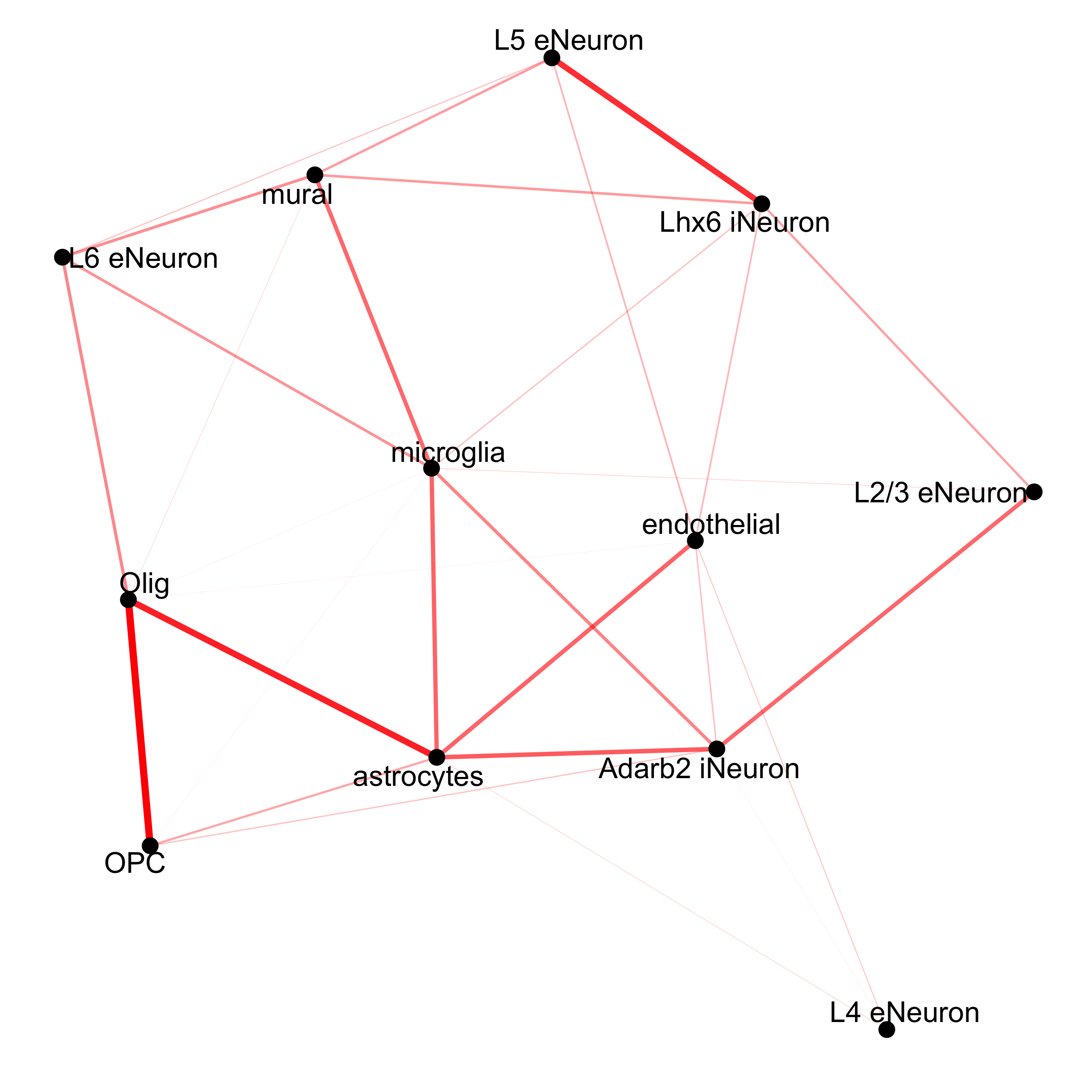
cellProximityNetwork(gobject = SS_seqfish, CPscore = cell_proximities, remove_self_edges = T,only_show_enrichment_edges = T,save_param = c(save_name = '12_c_network_cell_cell_enrichment'))
## network with self-edges
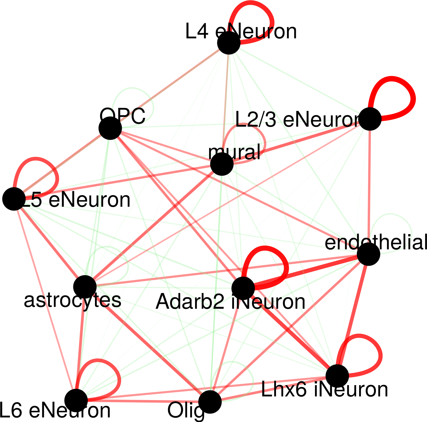
cellProximityNetwork(gobject = SS_seqfish, CPscore = cell_proximities,remove_self_edges = F, self_loop_strength = 0.3,only_show_enrichment_edges = F,rescale_edge_weights = T,node_size = 8,edge_weight_range_depletion = c(1, 2),edge_weight_range_enrichment = c(2,5),save_param = c(save_name = '12_d_network_cell_cell_enrichment_self',base_height = 5, base_width = 5, save_format = 'pdf'))
## visualization of specific cell types
# Option 1
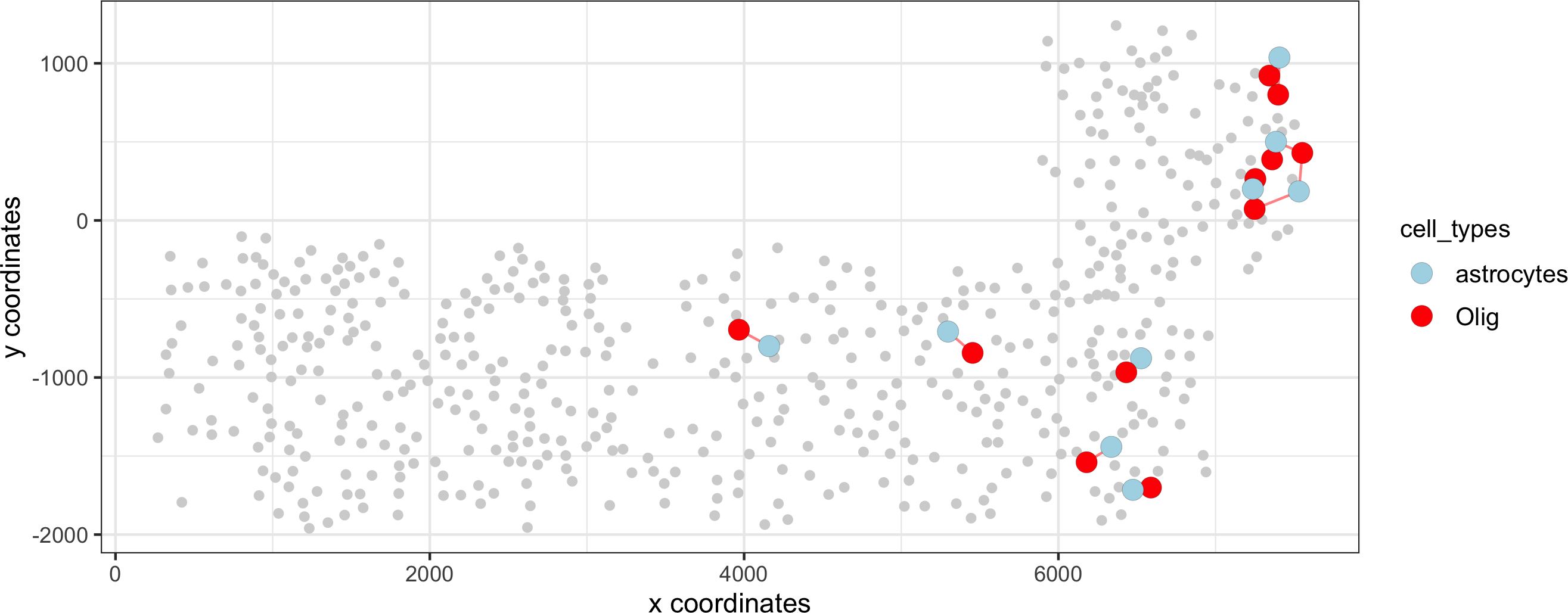
spec_interaction = "astrocytes--Olig"
cellProximitySpatPlot2D(gobject = SS_seqfish,interaction_name = spec_interaction,show_network = T,cluster_column = 'cell_types',cell_color = 'cell_types',cell_color_code = c(astrocytes = 'lightblue', Olig = 'red'),point_size_select = 4, point_size_other = 2,save_param = c(save_name = '12_e_cell_cell_enrichment_selected'))
# Option 2: create additional metadata
SS_seqfish = addCellIntMetadata(SS_seqfish, spatial_network = 'spatial_network',cluster_column = 'cell_types',cell_interaction = spec_interaction,name = 'astro_olig_ints')
spatPlot(SS_seqfish, cell_color = 'astro_olig_ints',select_cell_groups =  c('other_astrocytes', 'other_Olig', 'select_astrocytes', 'select_Olig'),legend_symbol_size = 3, save_param = c(save_name = '12_f_cell_cell_enrichment_sel_vs_not'))

12_a_barplot_cell_cell_enrichment.png

12_b_heatmap_cell_cell_enrichment.png

12_c_network_cell_cell_enrichment.png

12_d_network_cell_cell_enrichment_self.png

12_e_cell_cell_enrichment_selected.png

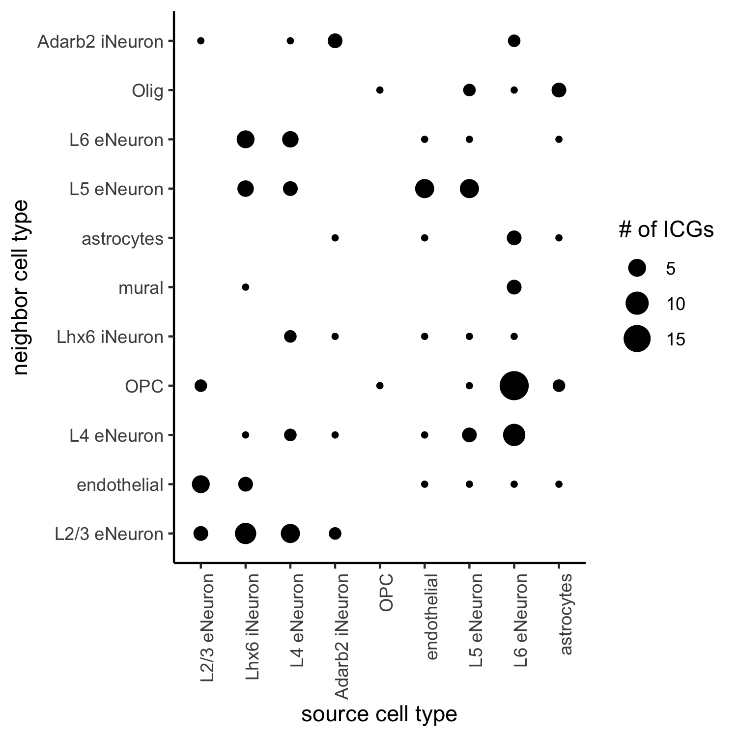
12.2. Cell neighborhood: interaction changed genes

## select top 25th highest expressing genes
gene_metadata = fDataDT(SS_seqfish)
plot(gene_metadata$nr_cells, gene_metadata$mean_expr)
plot(gene_metadata$nr_cells, gene_metadata$mean_expr_det)
quantile(gene_metadata$mean_expr_det)
high_expressed_genes = gene_metadata[mean_expr_det > 1.31]$gene_ID
## identify genes that are associated with proximity to other cell types
CPGscoresHighGenes =  findCPG(gobject = SS_seqfish,selected_genes = high_expressed_genes,spatial_network_name = 'Delaunay_network',cluster_column = 'cell_types',diff_test = 'permutation',adjust_method = 'fdr',nr_permutations = 2000, do_parallel = T, cores = 2)
## visualize all genes
plotCellProximityGenes(SS_seqfish, cpgObject = CPGscoresHighGenes, method = 'dotplot', save_param = c(save_name = '13_a_CPG_dotplot', base_width = 5, base_height = 5))
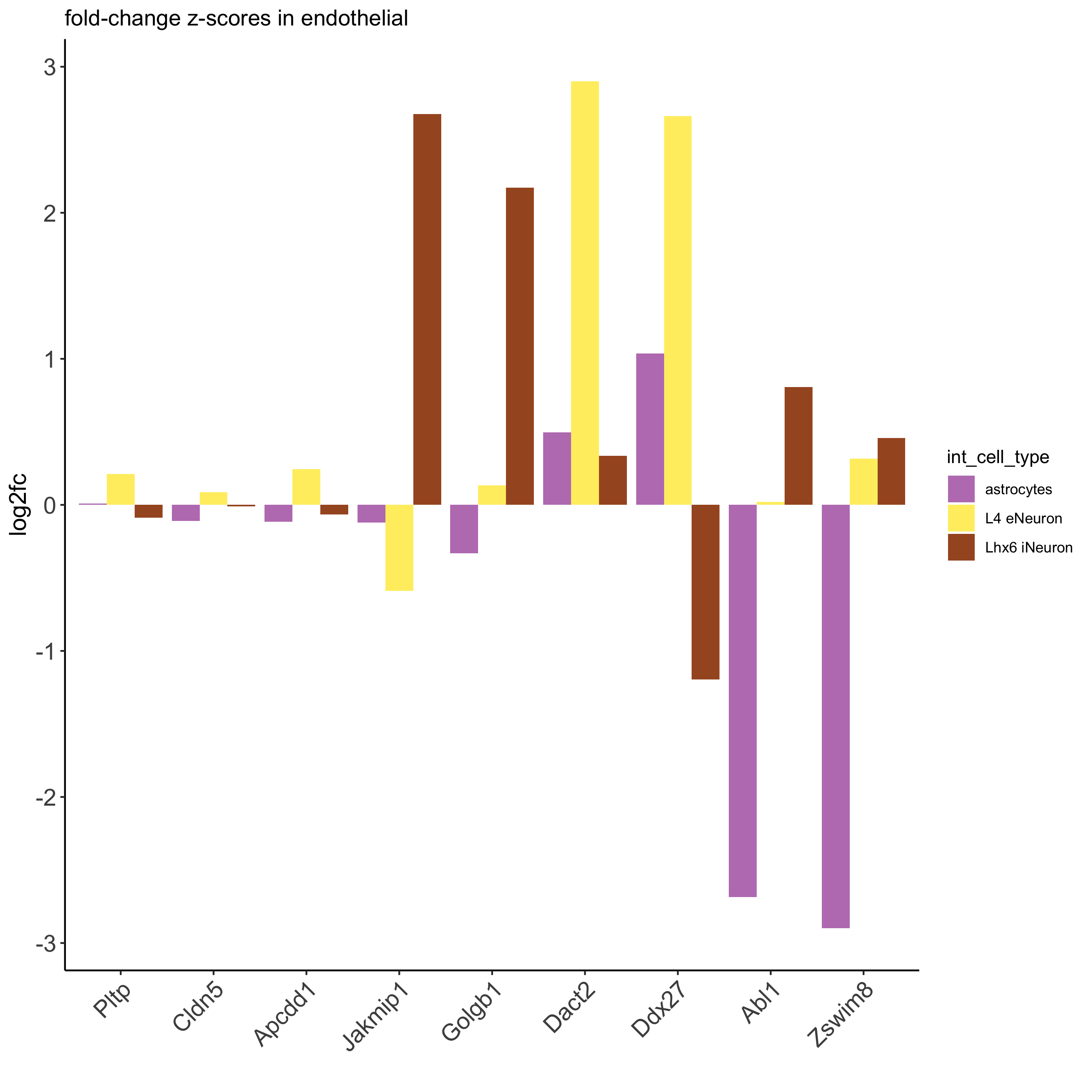
## filter genes
CPGscoresFilt = filterCPG(CPGscoresHighGenes)
## visualize subset of interaction changed genes (ICGs)
ICG_genes = c('Jakmip1', 'Golgb1', 'Dact2', 'Ddx27', 'Abl1', 'Zswim8')
ICG_genes_types = c('Lhx6 iNeuron', 'Lhx6 iNeuron', 'L4 eNeuron', 'L4 eNeuron', 'astrocytes', 'astrocytes')
names(ICG_genes) = ICG_genes_types
plotICG(gobject = SS_seqfish,cpgObject = CPGscoresHighGenes,source_type = 'endothelial',source_markers = c('Pltp', 'Cldn5', 'Apcdd1'),ICG_genes = ICG_genes,save_param = c(save_name = '13_b_ICG_barplot'))

13_a_CPG_dotplot.png

13_b_ICG_barplot.png

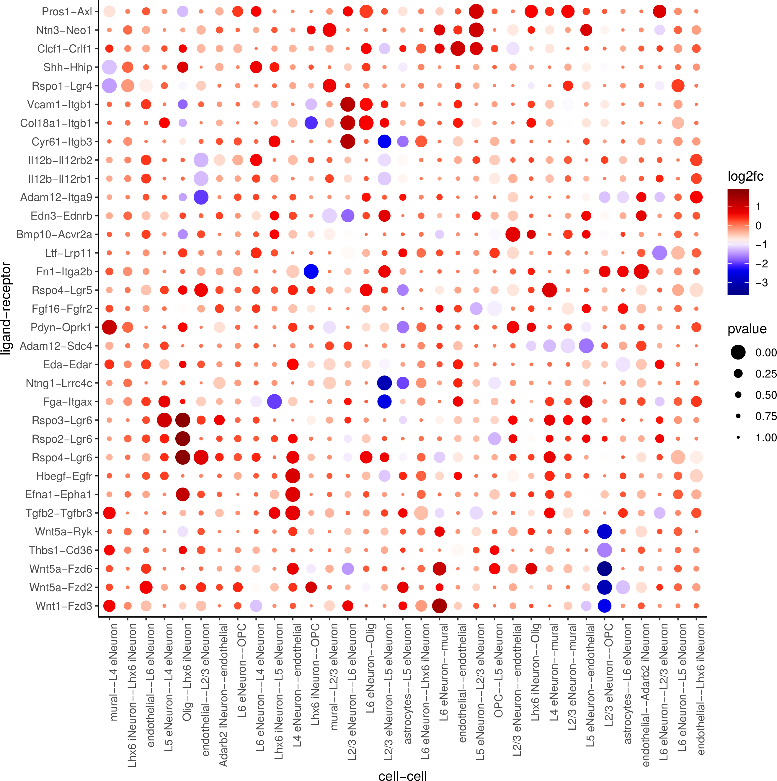
12.3. Cell neighborhood: ligand-receptor cell-cell communication

# LR expression
# LR activity changes
LR_data = data.table::fread(system.file("extdata", "mouse_ligand_receptors.txt", package = 'Giotto'))
LR_data[, ligand_det := ifelse(mouseLigand %in% SS_seqfish@gene_ID, T, F)]
LR_data[, receptor_det := ifelse(mouseReceptor %in% SS_seqfish@gene_ID, T, F)]
LR_data_det = LR_data[ligand_det == T & receptor_det == T]
select_ligands = LR_data_det$mouseLigand
select_receptors = LR_data_det$mouseReceptor
## get statistical significance of gene pair expression changes based on expression
expr_only_scores = exprCellCellcom(gobject = SS_seqfish,cluster_column = 'cell_types', random_iter = 1000,gene_set_1 = select_ligands,gene_set_2 = select_receptors)
## get statistical significance of gene pair expression changes upon cell-cell interaction
spatial_all_scores = spatCellCellcom(SS_seqfish,spatial_network_name = 'spatial_network',cluster_column = 'cell_types', random_iter = 1000,gene_set_1 = select_ligands,gene_set_2 = select_receptors,adjust_method = 'fdr',do_parallel = T,cores = 2, verbose = 'a little')
## select top LR ##
selected_spat = spatial_all_scores[p.adj <= 0.01 & abs(log2fc) > 0.25 & lig_nr >= 4 & rec_nr >= 4]
data.table::setorder(selected_spat, -PI)
top_LR_ints = unique(selected_spat[order(-abs(PI))]$LR_comb)[1:33]
top_LR_cell_ints = unique(selected_spat[order(-abs(PI))]$LR_cell_comb)[1:33]
plotCCcomDotplot(gobject = SS_seqfish,comScores = spatial_all_scores,selected_LR = top_LR_ints,selected_cell_LR = top_LR_cell_ints,cluster_on = 'PI',save_param = c(save_name = '14_a_communication_dotplot', save_format = 'pdf'))
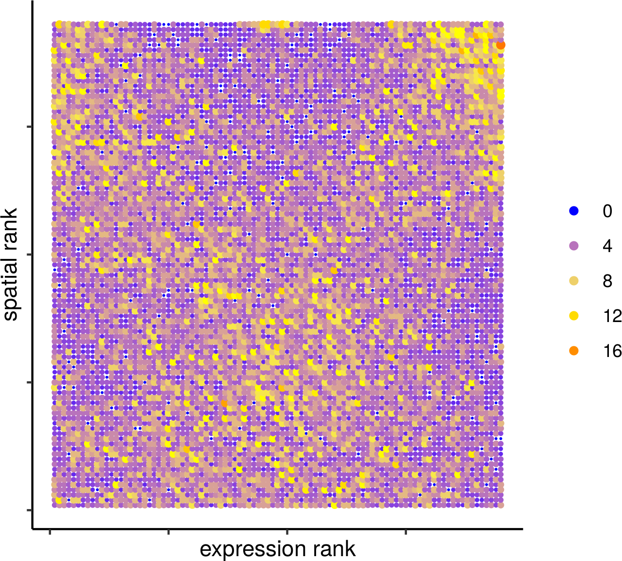
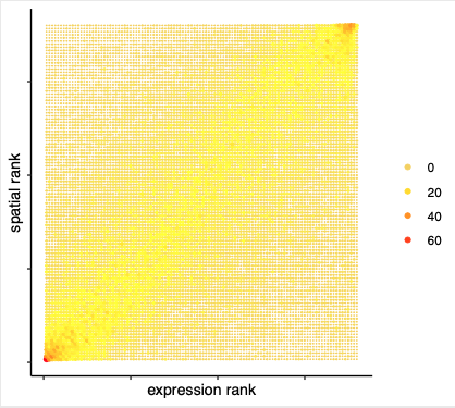
## spatial vs rank ####
comb_comm = combCCcom(spatialCC = spatial_all_scores,exprCC = expr_only_scores)
# top differential activity levels for ligand receptor pairs
plotRankSpatvsExpr(gobject = SS_seqfish,comb_comm,expr_rnk_column = 'exprPI_rnk',spat_rnk_column = 'spatPI_rnk',midpoint = 10,save_param = c(save_name = '14_b_expr_vs_spatial_activity',base_height = 4, base_width = 4.5, save_format = 'pdf'))
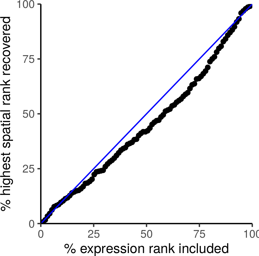
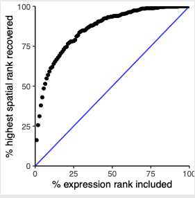
## recovery ####
## predict maximum differential activity
plotRecovery(gobject = SS_seqfish,comb_comm,expr_rnk_column = 'exprPI_rnk',spat_rnk_column = 'spatPI_rnk',ground_truth = 'spatial',save_param = c(save_name = '14_c_spatial_recovery_activity', base_height = 3, base_width = 3, save_format = 'pdf'))

14_a_communication_dotplot.png

14_b_expr_vs_spatial_activity.png

14_c_spatial_recovery_activity.png

# highest levels of ligand and receptor prediction
# top differential activity levels for ligand receptor pairs
plotRankSpatvsExpr(gobject = SS_seqfish, comb_comm, expr_rnk_column = 'LR_expr_rnk', spat_rnk_column = 'LR_spat_rnk', midpoint = 10, save_param = c(save_name = '14_b_expr_vs_spatial_expression_rank', base_height = 4, base_width = 4.5, save_format = 'pdf'))
plotRecovery(gobject = SS_seqfish,comb_comm, expr_rnk_column = 'LR_expr_rnk',spat_rnk_column = 'LR_spat_rnk',ground_truth = 'spatial',save_param = c(save_name = '14_c_spatial_recovery_expression_rank', base_height = 3, base_width = 3, save_format = 'pdf'))

14_b_expr_vs_spatial_expression_rank.png

14_c_spatial_recovery_expression_rank.png

13. Export Giotto Analyzer to Viewer

viewer_folder = fs::path(my_working_dir, 'Mouse_cortex_viewer')
# select annotations, reductions and expression values to view in Giotto Viewer
pDataDT(SS_seqfish)
exportGiottoViewer(gobject = SS_seqfish, output_directory = viewer_folder,factor_annotations =c('cell_types','leiden_clus','sub_leiden_clus_select','HMRF_2_k9_b.28'),numeric_annotations = 'total_expr',dim_reductions = c('umap'),dim_reduction_names = c('umap'),expression_values = 'scaled',expression_rounding = 3,overwrite_dir = TRUE)

#================================================================ 
#Next steps. Please manually run the following in a SHELL terminal: 
#================================================================ 
cd  /data/Mouse_cortex_viewer 
giotto_setup_image --require-stitch=n --image=n --image-multi-channel=n --segmentation=n --multi-fov=n --output-json=step1.json 
smfish_step1_setup -c step1.json 
giotto_setup_viewer --num-panel=2 --input-preprocess-json=step1.json --panel-1=PanelPhysicalSimple --panel-2=PanelTsne --output-json=step2.json --input-annotation-list=annotation_list.txt 
smfish_read_config -c step2.json -o test.dec6.js -p test.dec6.html -q test.dec6.css 
giotto_copy_js_css --output . 
python3 -m http.server 
================================================================ 
#Finally, open your browser, navigate to http://localhost:8000/. Then click on the file test.dec6.html to see the viewer.