CyCIF dataset

0. Environment

library(Giotto)
# STOP!
# ====== 1. set working directory ======
# For Docker, set my_working_dir to /data
my_working_dir = '/data'
# For native install users, set my_working_dir to a directory accessible by user
#my_working_dir = "/home/qzhu/Downloads"
# ====== 2. set giotto python path ======
# For Docker, set python_path to /usr/bin/python3
python_path = "/usr/bin/python3"
# For native install users, python path may be different, and may depend on whether conda or virtual environment. One can check by "reticulate::py_discover_config()" to see which python is picked up automatically. Then set python_path to what is returned by py_discover_config.
# python_path = "/usr/bin/python3"

1. Dataset preparation

1.1. Dataset explanation

The CyCIF data to run this tutorial can be found here. Alternatively you can use the getSpatialDataset to automatically download this dataset like we do in this example.

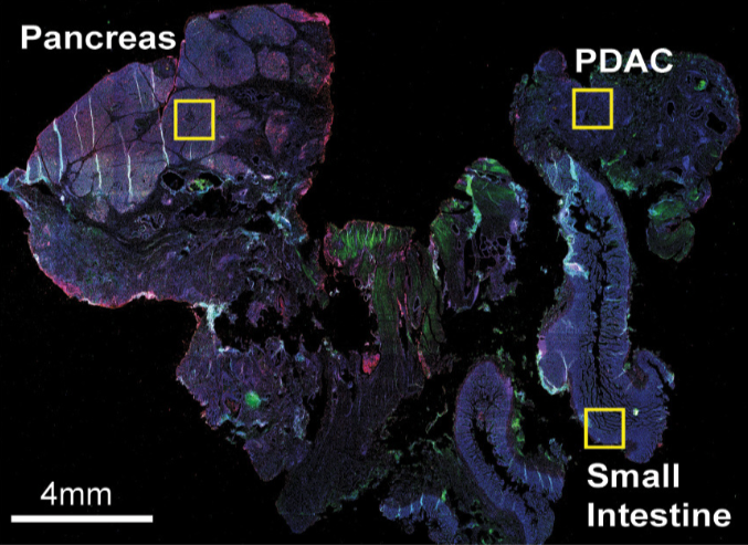
We will re-analyze the PDAC data generated by tissue-CyCIF as explained in the paper by Lin et al.

1.2. Dataset download

# download data to working directory ####
# if wget is installed, set method = 'wget'
getSpatialDataset(dataset = 'cycif_PDAC', directory = my_working_dir, method = 'wget')

1.3 Giotto global instructions and preparations

# 1. (optional) set Giotto instructions
instrs = createGiottoInstructions(save_plot = TRUE,show_plot = FALSE,save_dir = my_working_dir, python_path=python_path)
# 2. create giotto object from provided paths ####
expr_path = fs::path(my_working_dir, "cyCIF_PDAC_expression.txt.gz")
loc_path = fs::path(my_working_dir, "cyCIF_PDAC_coord.txt")
meta_path = fs::path(my_working_dir, "cyCIF_PDAC_annot.txt")
png_path = fs::path(my_working_dir, "canvas.png")

2. Create Giotto object & process data

# read in data information
# expression info
pdac_expression = readExprMatrix(expr_path, transpose = T)
# cell coordinate info
pdac_locations = data.table::fread(loc_path)
# metadata
pdac_metadata = data.table::fread(meta_path)
pdac_test <- createGiottoObject(raw_exprs = pdac_expression, 
spatial_locs = pdac_locations,instructions = instrs,cell_metadata = pdac_metadata)
## normalize & adjust
pdac_test <- normalizeGiotto(gobject = pdac_test, scalefactor = 10000, verbose = T)
pdac_test <- addStatistics(gobject = pdac_test)
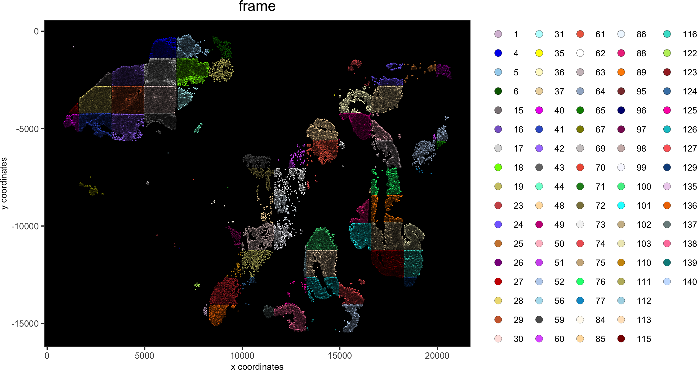
## visualize original annotations ##
spatPlot(gobject = pdac_test, point_size = 0.5, coord_fix_ratio = 1, cell_color = 'frame',background_color = 'black', legend_symbol_size = 3,save_param = list(save_name = '2_a_spatPlot'))

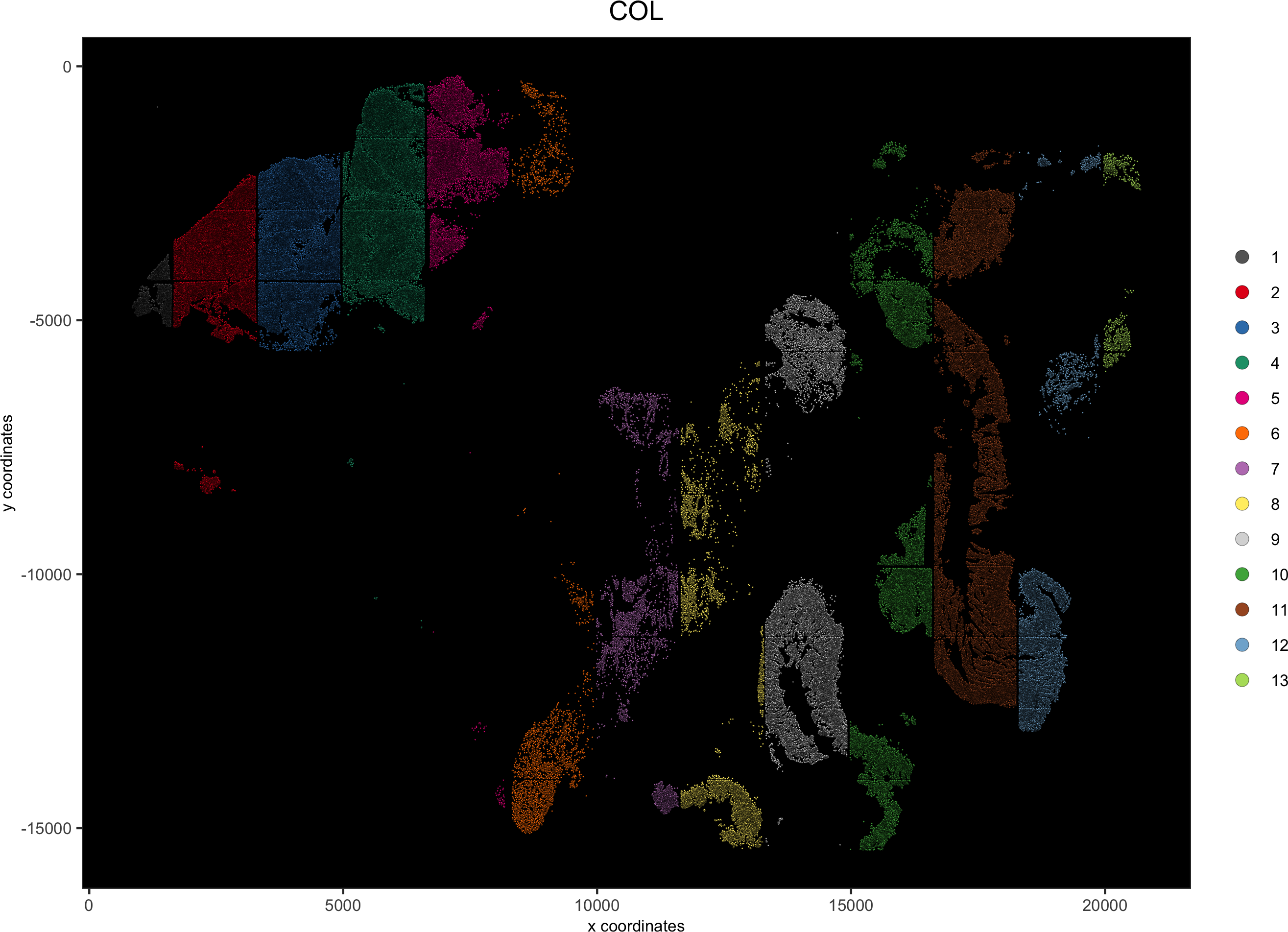
spatPlot(gobject = pdac_test, point_size = 0.3, coord_fix_ratio = 1, 
cell_color = 'COL', background_color = 'black', legend_symbol_size = 3,save_param = list(save_name = '2_b_spatPlot_column'))

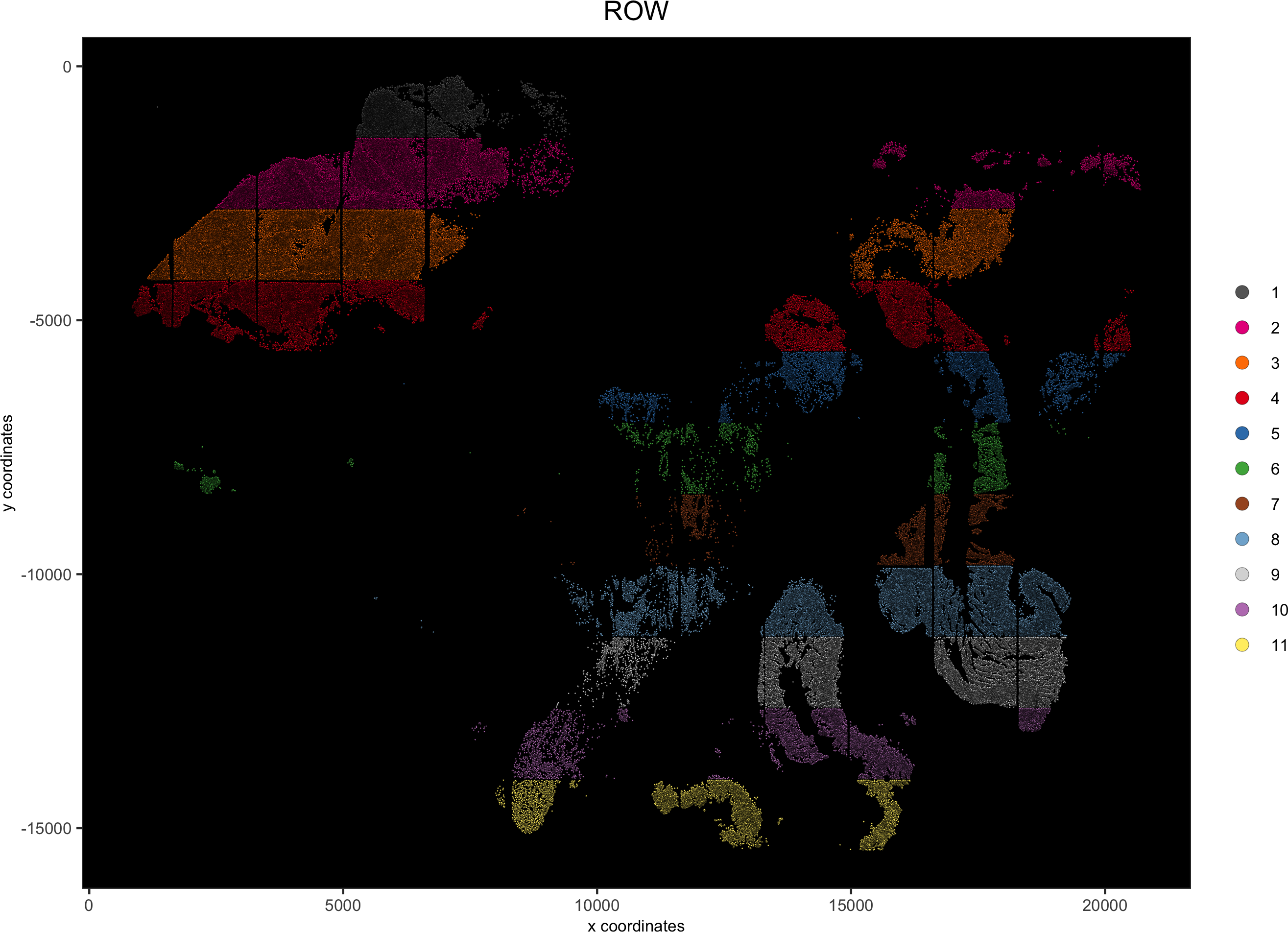
spatPlot(gobject = pdac_test, point_size = 0.3, coord_fix_ratio = 1, 
cell_color = 'ROW', background_color = 'black', legend_symbol_size = 3,save_param = list(save_name = '2_c_spatPlot_row'))

## add external histology information
pdac_metadata = pDataDT(pdac_test)
pancreas_frames = c(1:6, 27:31, 15:19, 40:44)
PDAC_frames = c(23:26, 35:37, 51:52, 64:65, 77)
small_intestines_frames = c(49:50, 63, 75:76, 88:89, 100:103, 112:116, 125:129, 137:140)
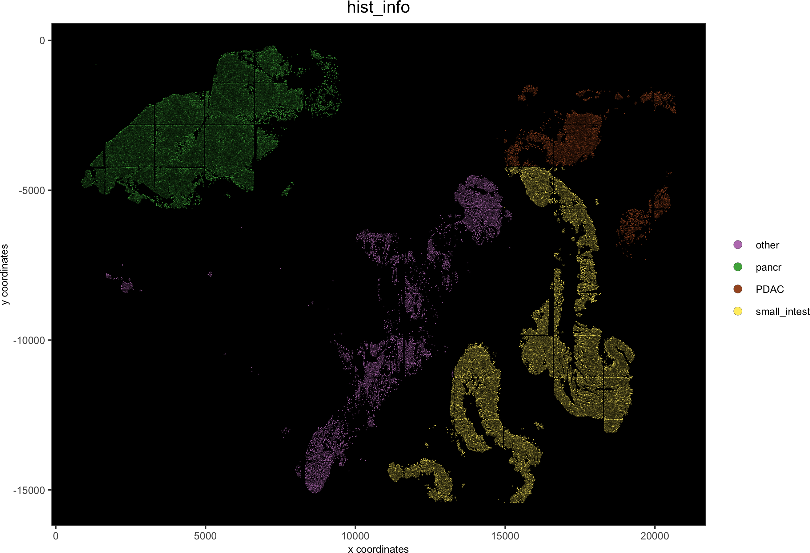
# detailed histology
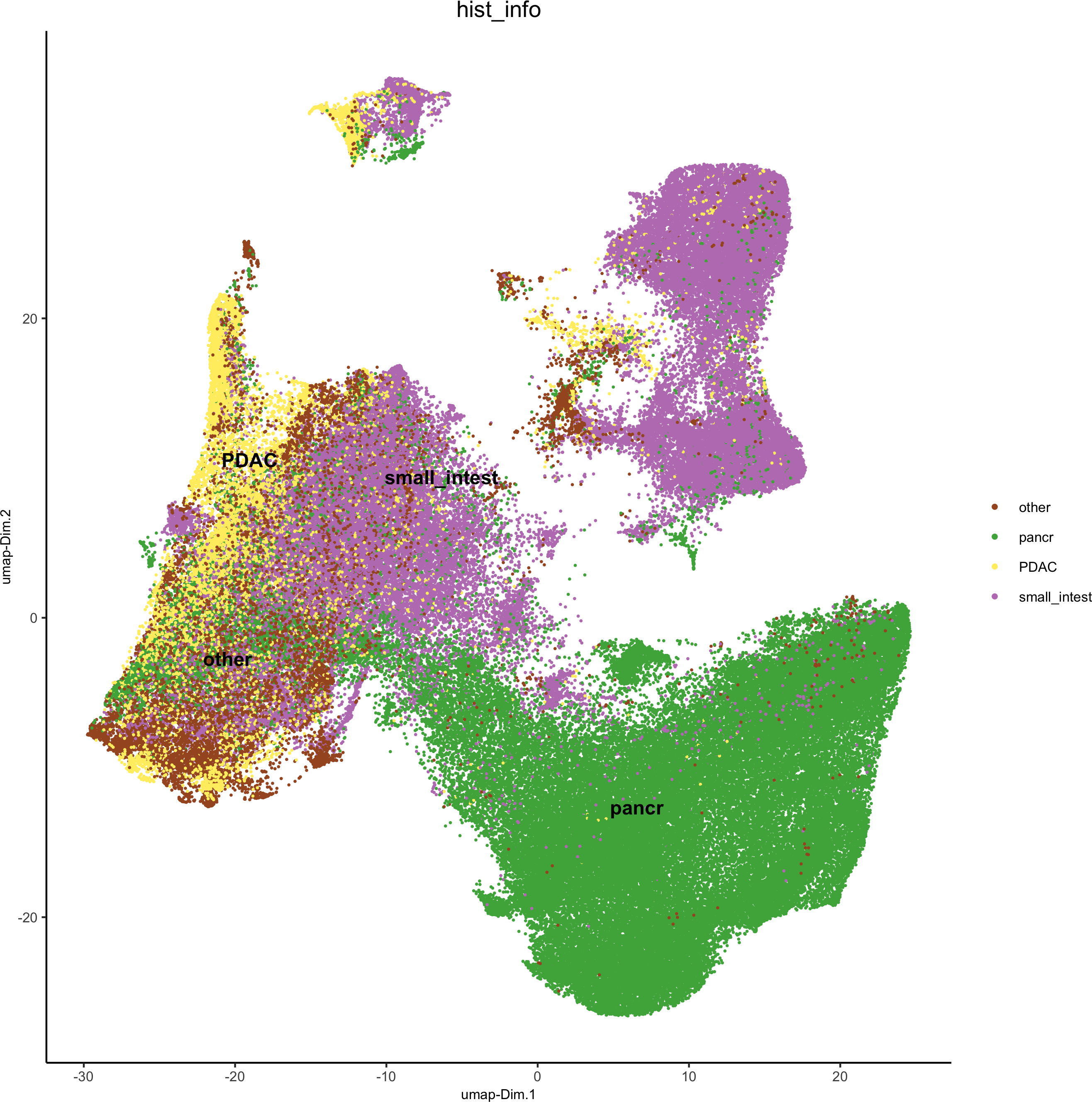
hist_info = ifelse(pdac_metadata$frame %in% pancreas_frames, 'pancr', 
ifelse(pdac_metadata$frame %in% PDAC_frames, 'PDAC',ifelse(pdac_metadata$frame %in% small_intestines_frames, 'small_intest', 'other')))
pdac_test = addCellMetadata(pdac_test, new_metadata = hist_info)
spatPlot(gobject = pdac_test, point_size = 0.3, coord_fix_ratio = 1, cell_color = 'hist_info',background_color = 'black', legend_symbol_size = 3,save_param = list(save_name = '2_d_spatPlot_hist'))

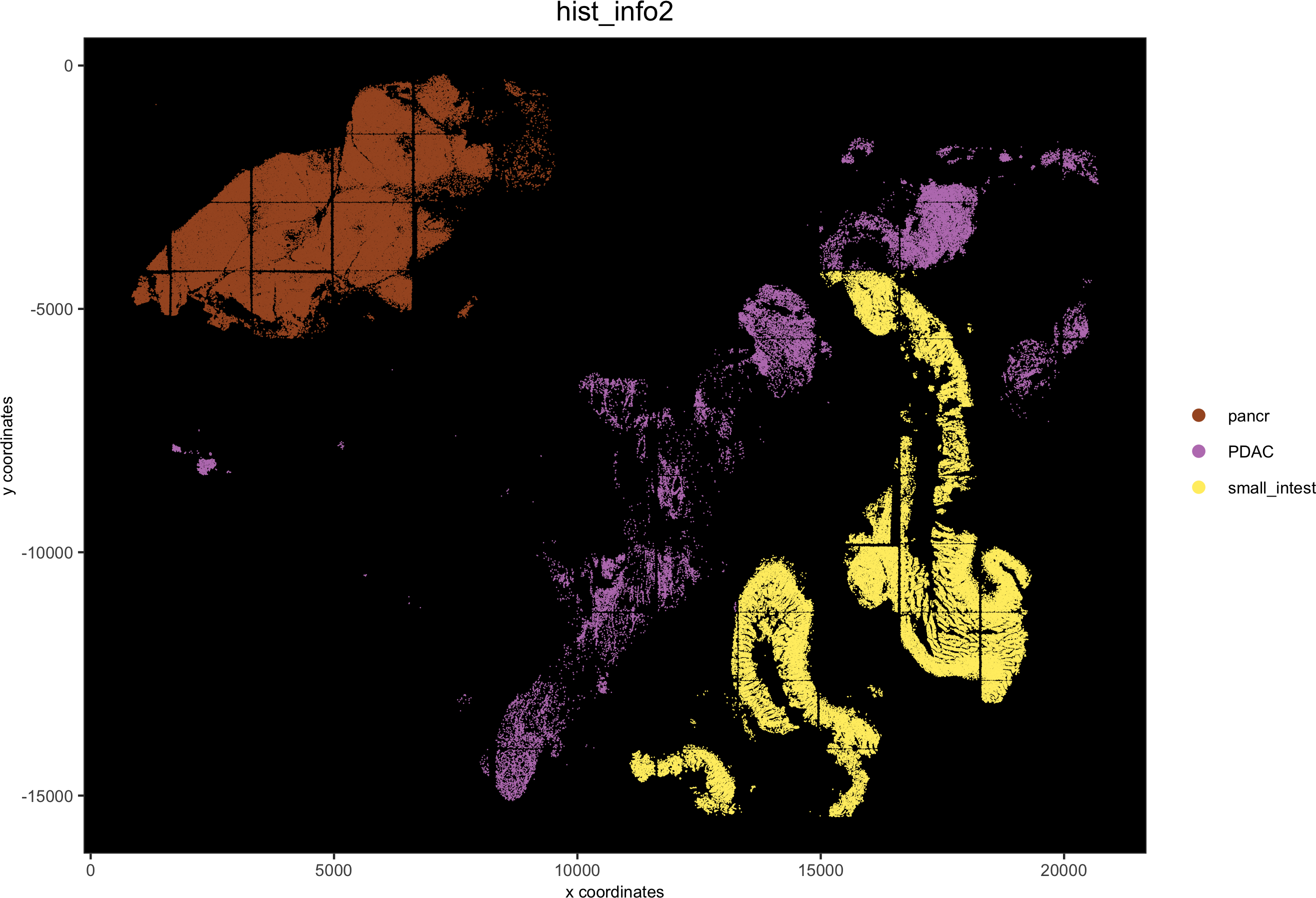
# coarse histology
hist_info2 = ifelse(pdac_metadata$frame %in% pancreas_frames, 'pancr', 
ifelse(pdac_metadata$frame %in% small_intestines_frames, 'small_intest','PDAC'))
pdac_test = addCellMetadata(pdac_test, new_metadata = hist_info2)
spatPlot(gobject = pdac_test, point_size = 0.3, coord_fix_ratio = 1, cell_color = 'hist_info2',background_color = 'black', legend_symbol_size = 3, point_border_stroke = 0.001,save_param = list(save_name = '2_e_spatPlot_hist2'))

2.1. Add and align image:

1. read image with magick
   
2. modify image optional (e.g. flip axis, negate, change background, ...)
   
3. test if image is aligned
   

# read
mg_img = magick::image_read(png_path)
# flip/flop (convert x and y axes)
mg_img = magick::image_flip(mg_img)
mg_img = magick::image_flop(mg_img)
# negate image
mg_img2 = magick::image_negate(mg_img)
## align image ##
# 1. create spatplot
mypl = spatPlot(gobject = pdac_test, point_size = 0.3, coord_fix_ratio = NULL, cell_color = 'hist_info2',legend_symbol_size = 3, point_border_stroke = 0.001,save_plot = F, return_plot = T)
# 2.create giotto image and make adjustments (xmax_adj, xmin_adj, ...)
hist_png = createGiottoImage(gobject = pdac_test, mg_object = mg_img2, name = 'image_hist',xmax_adj = 5000, xmin_adj = 2500, ymax_adj = 1500, ymin_adj = 1500)
# 3. add giotto image to spatplot to check alignment
mypl_image = addGiottoImageToSpatPlot(mypl, hist_png)

1. add giotto image(s) to giotto object to call them within spat functions

## add images to Giotto object ##
image_list = list(hist_png)
pdac_test = addGiottoImage(gobject = pdac_test,images = image_list)
showGiottoImageNames(pdac_test)

3. Dimension reduction

# PCA
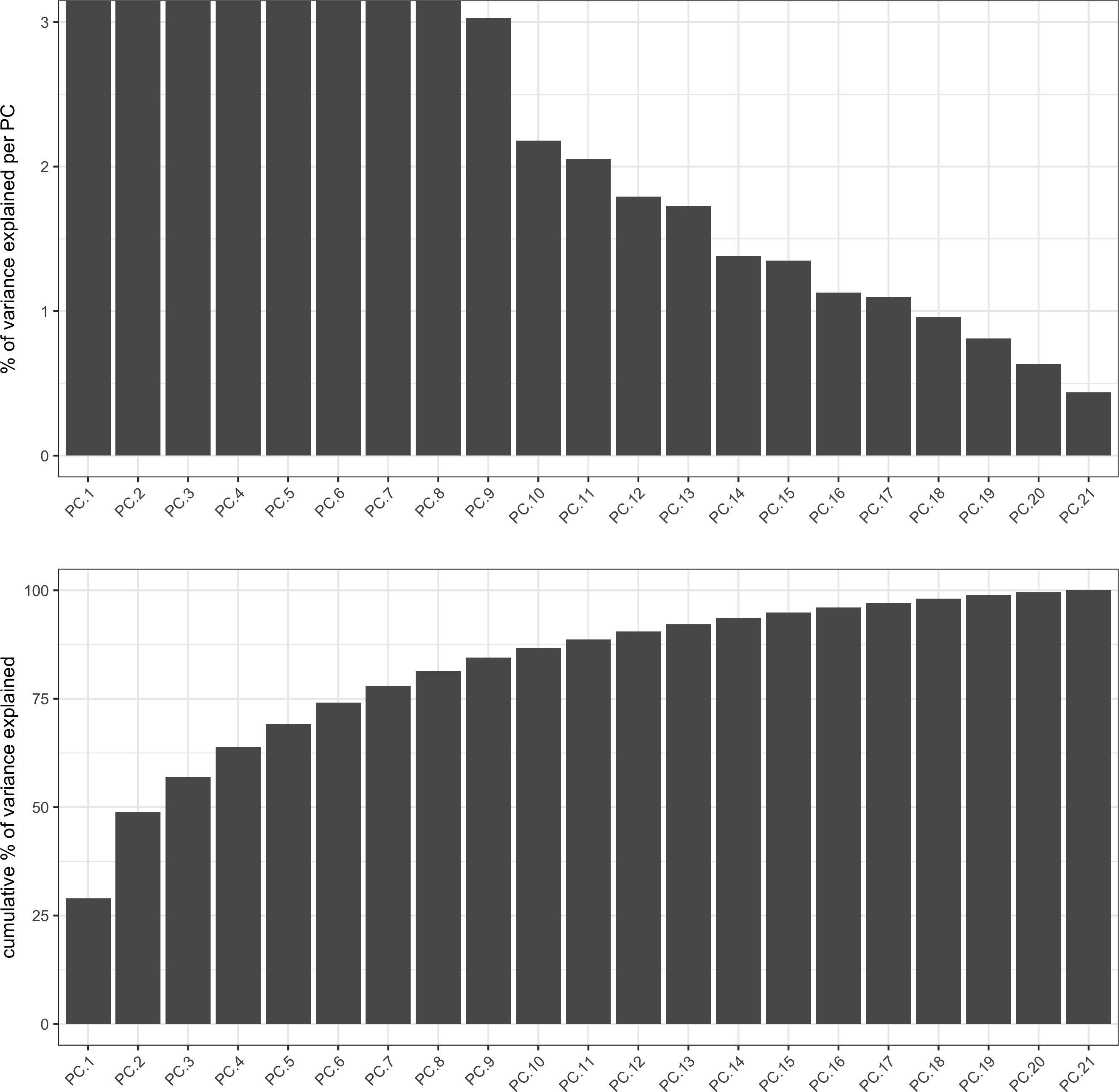
pdac_test <- runPCA(gobject = pdac_test, expression_values = 'normalized',scale_unit = T, center = F, method = 'factominer')
signPCA(pdac_test, scale_unit = T, scree_ylim = c(0, 3),save_param = list(save_name = '3_a_signPCA'))

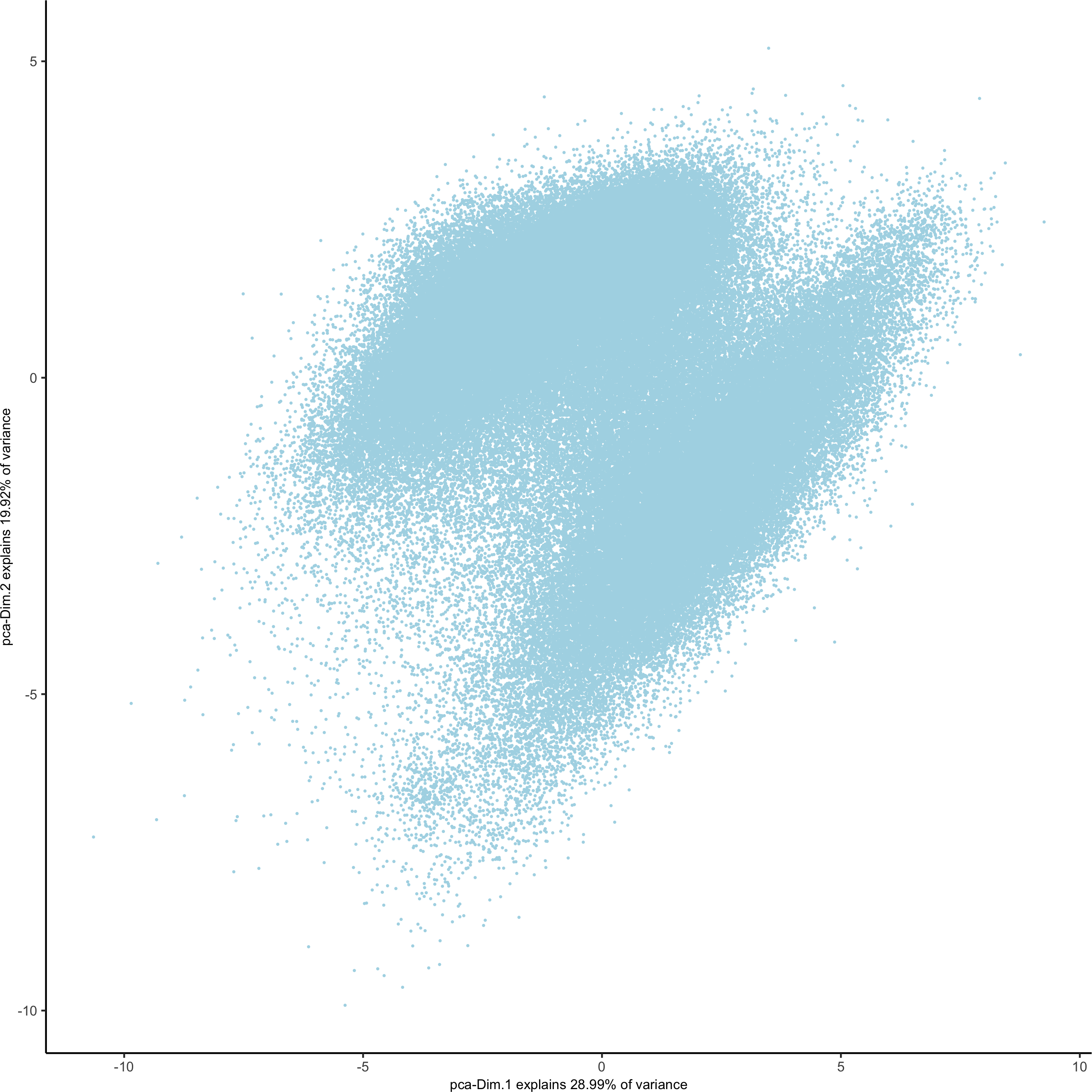
plotPCA(gobject = pdac_test, point_shape = 'no_border', point_size = 0.2, 
save_param = list(save_name = '3_b_PCAplot'))

# UMAP
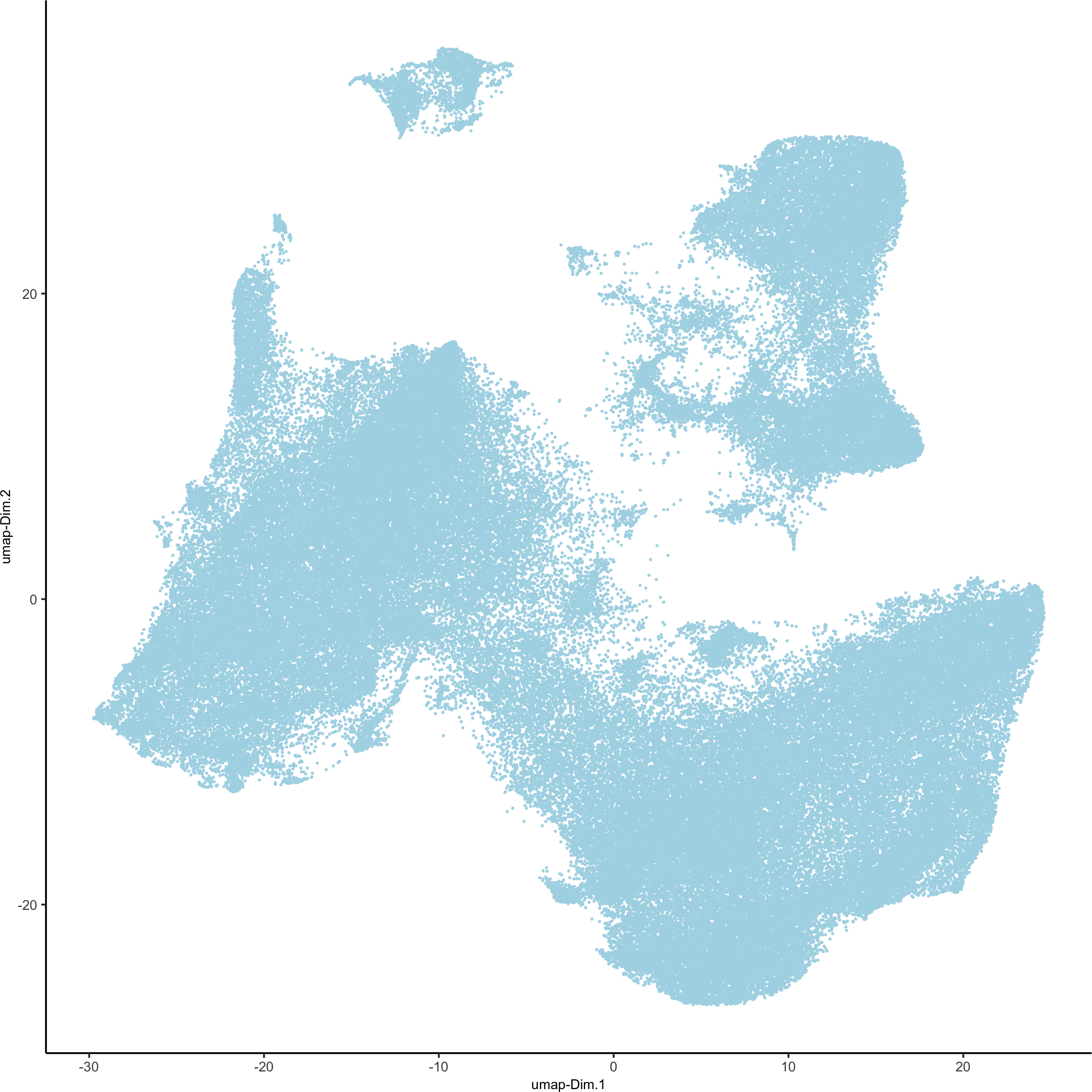
pdac_test <- runUMAP(pdac_test, dimensions_to_use = 1:14, n_components = 2, n_threads = 12)
plotUMAP(gobject = pdac_test, point_shape = 'no_border', point_size = 0.2,save_param = list(save_name = '3_c_UMAP'))

4. Clustering

## sNN network (default)
pdac_test <- createNearestNetwork(gobject = pdac_test, dimensions_to_use = 1:14, k = 20)
## 0.2 resolution
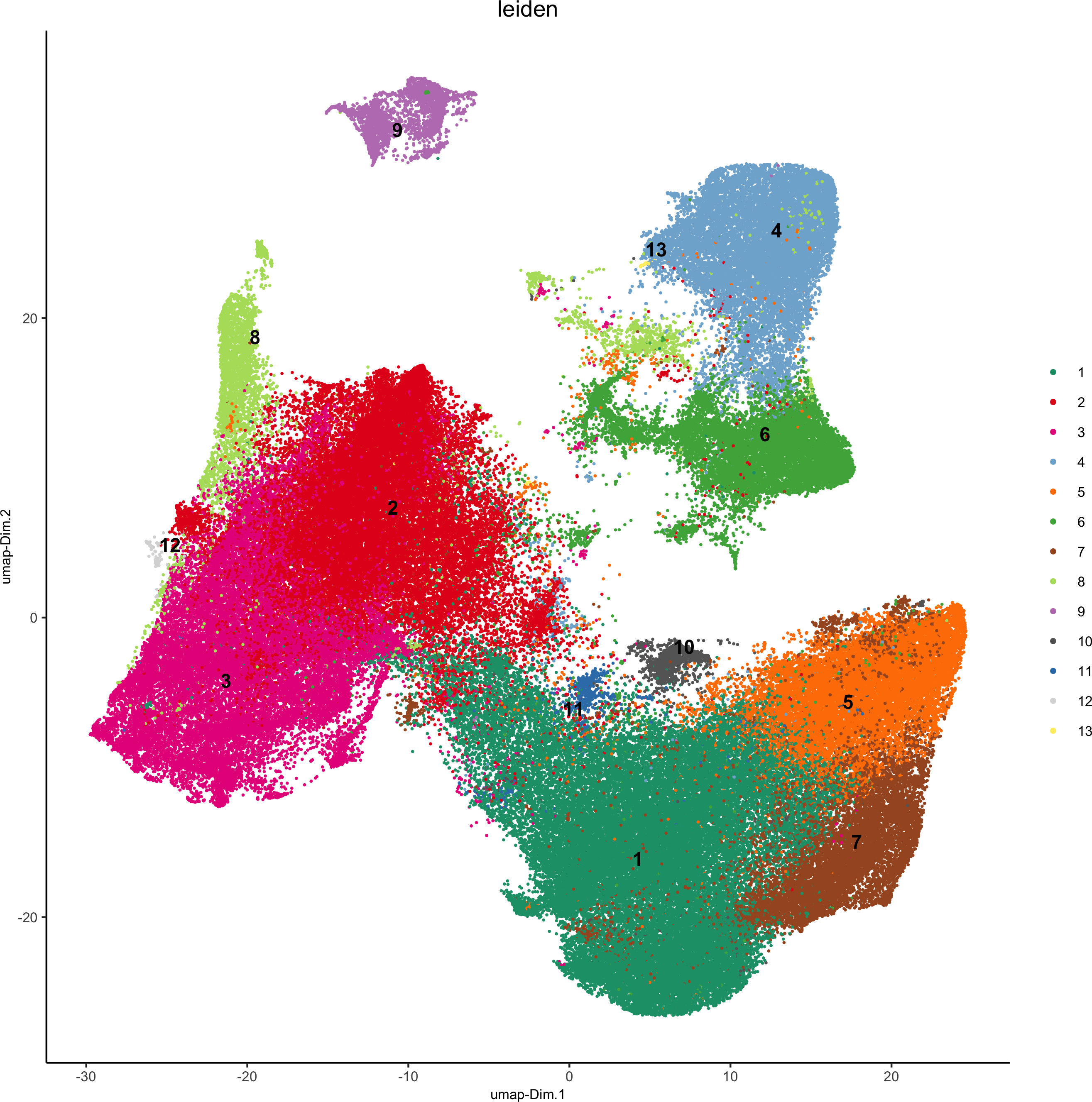
pdac_test <- doLeidenCluster(gobject = pdac_test, resolution = 0.2, n_iterations = 100, name = 'leiden')
# create customized color palette for leiden clustering results
pdac_metadata = pDataDT(pdac_test)
leiden_colors = Giotto:::getDistinctColors(length(unique(pdac_metadata$leiden)))
names(leiden_colors) = unique(pdac_metadata$leiden)
color_3 = leiden_colors['3'];color_10 = leiden_colors['10']
leiden_colors['3'] = color_10; leiden_colors['10'] = color_3
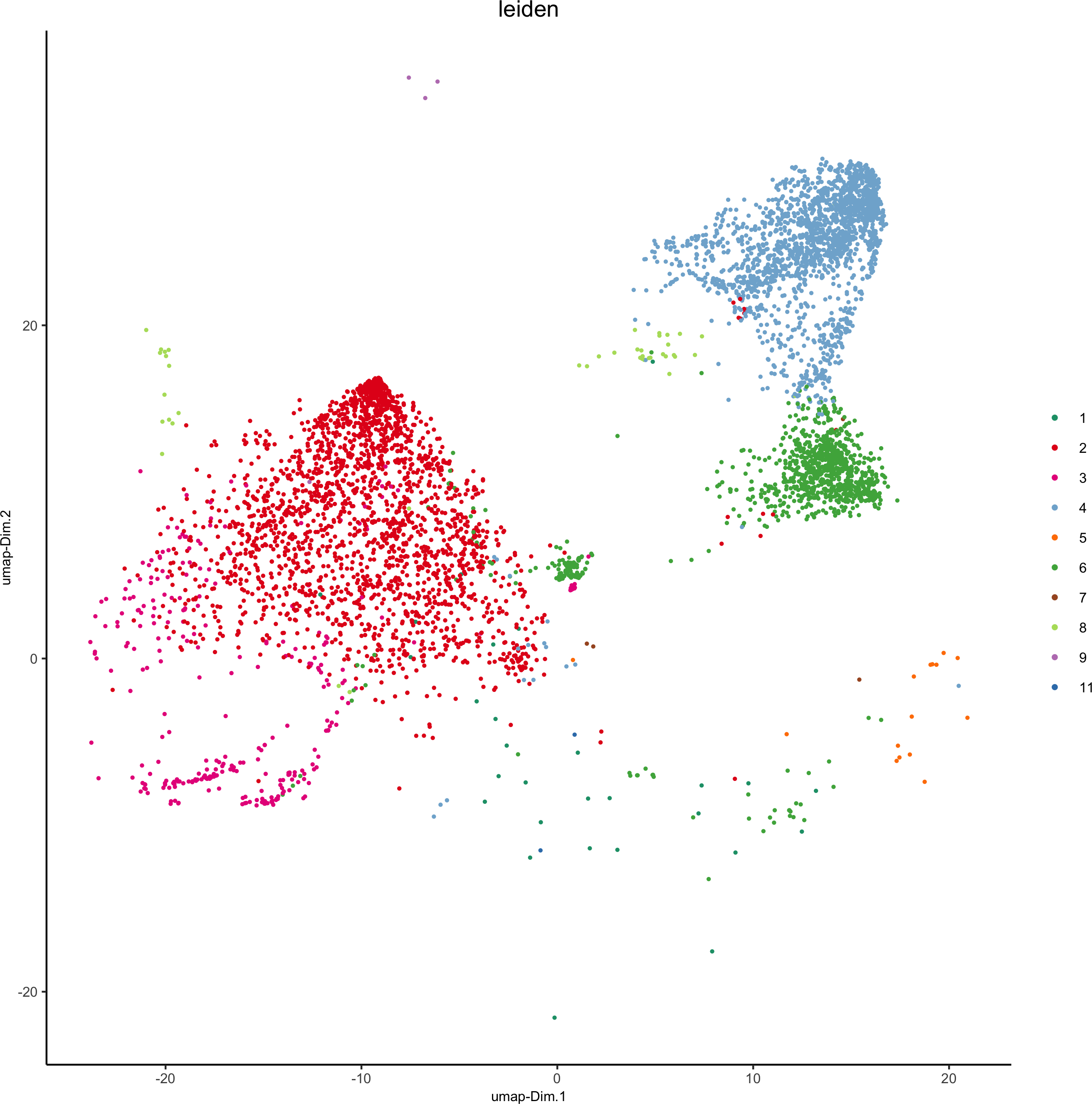
plotUMAP(gobject = pdac_test, cell_color = 'leiden', point_shape = 'no_border', 
point_size = 0.2, cell_color_code = leiden_colors,save_param = list(save_name = '4_a_UMAP'))

plotUMAP(gobject = pdac_test, cell_color = 'hist_info',point_shape = 'no_border',   point_size = 0.2,save_param = list(save_name = '4_b_UMAP'))

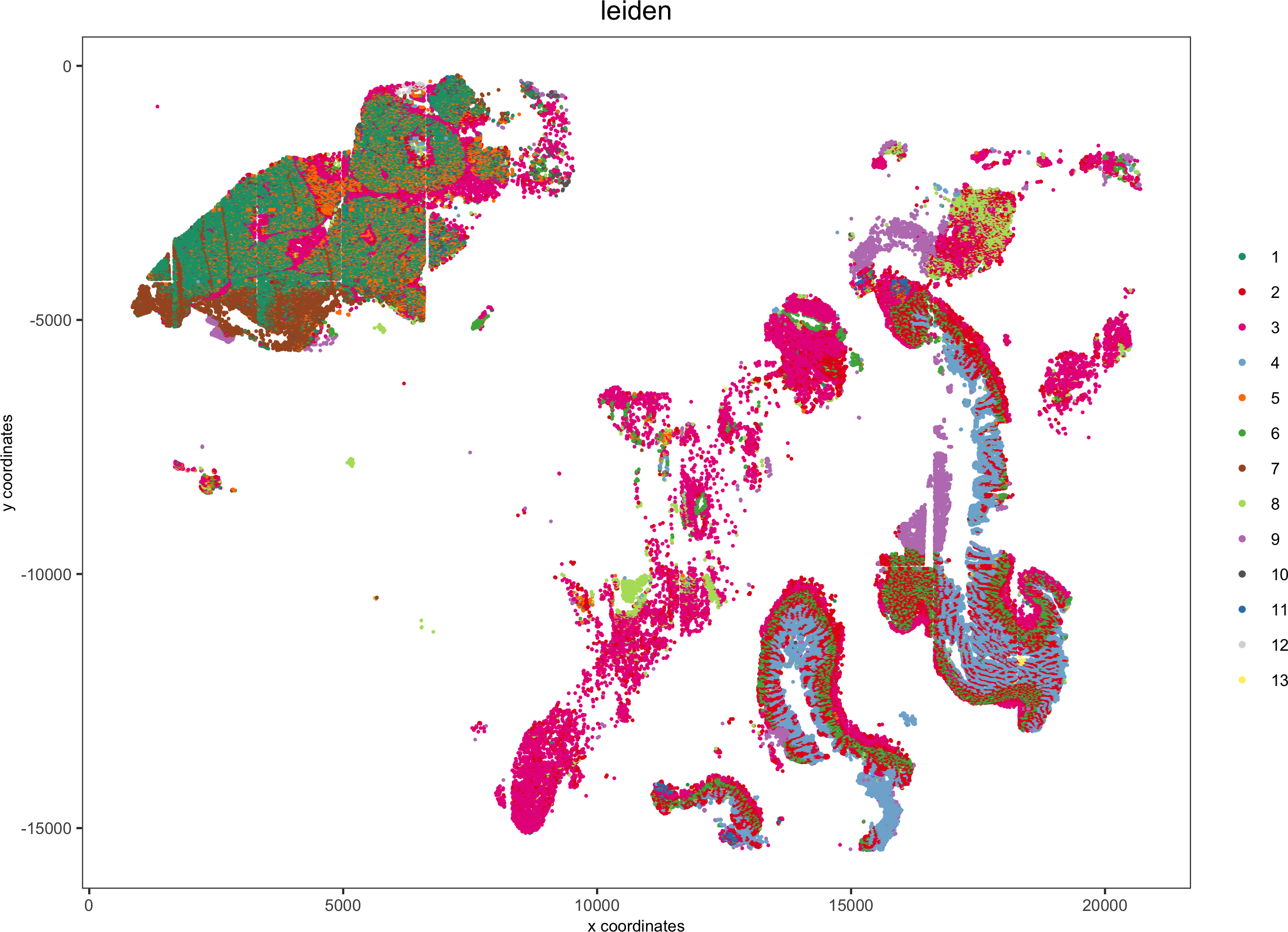
spatPlot(gobject = pdac_test, cell_color = 'leiden', point_shape = 'no_border', point_size = 0.2, 
cell_color_code = leiden_colors, coord_fix_ratio = 1,save_param = list(save_name = '4_c_spatplot'))

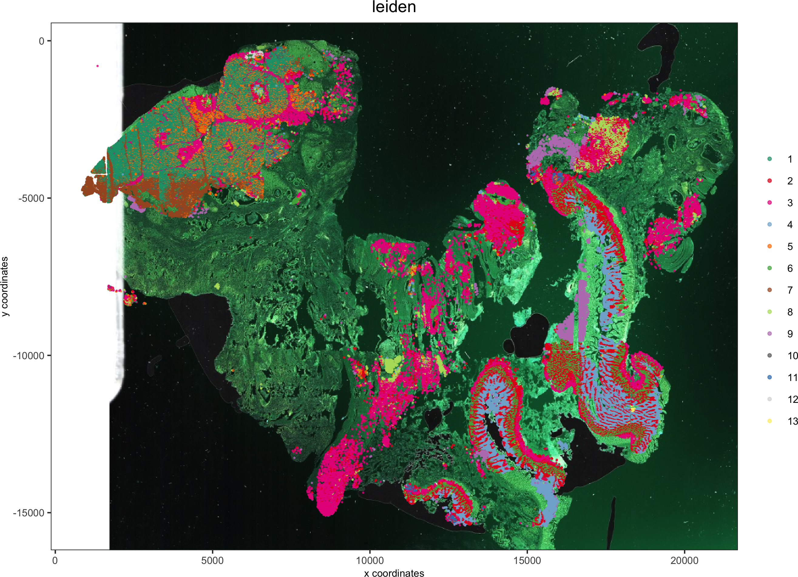
Add background image:

showGiottoImageNames(pdac_test)
spatPlot(gobject = pdac_test, show_image = T, image_name = 'image_hist',cell_color = 'leiden',point_shape = 'no_border', point_size = 0.2, point_alpha = 0.7, 
cell_color_code = leiden_colors, coord_fix_ratio = 1,save_param = list(save_name = '4_d_spatPlot'))

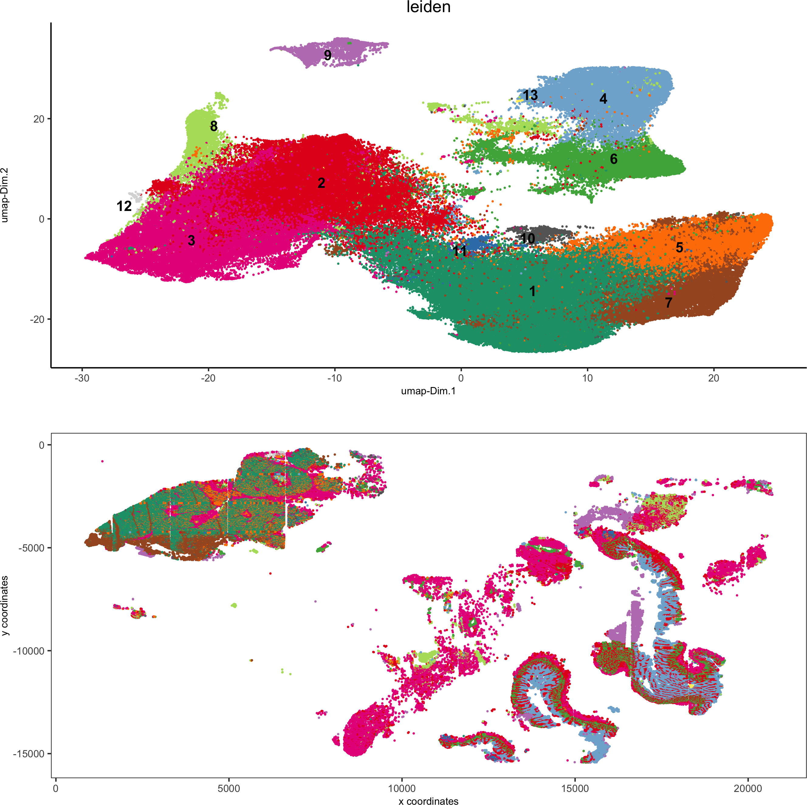
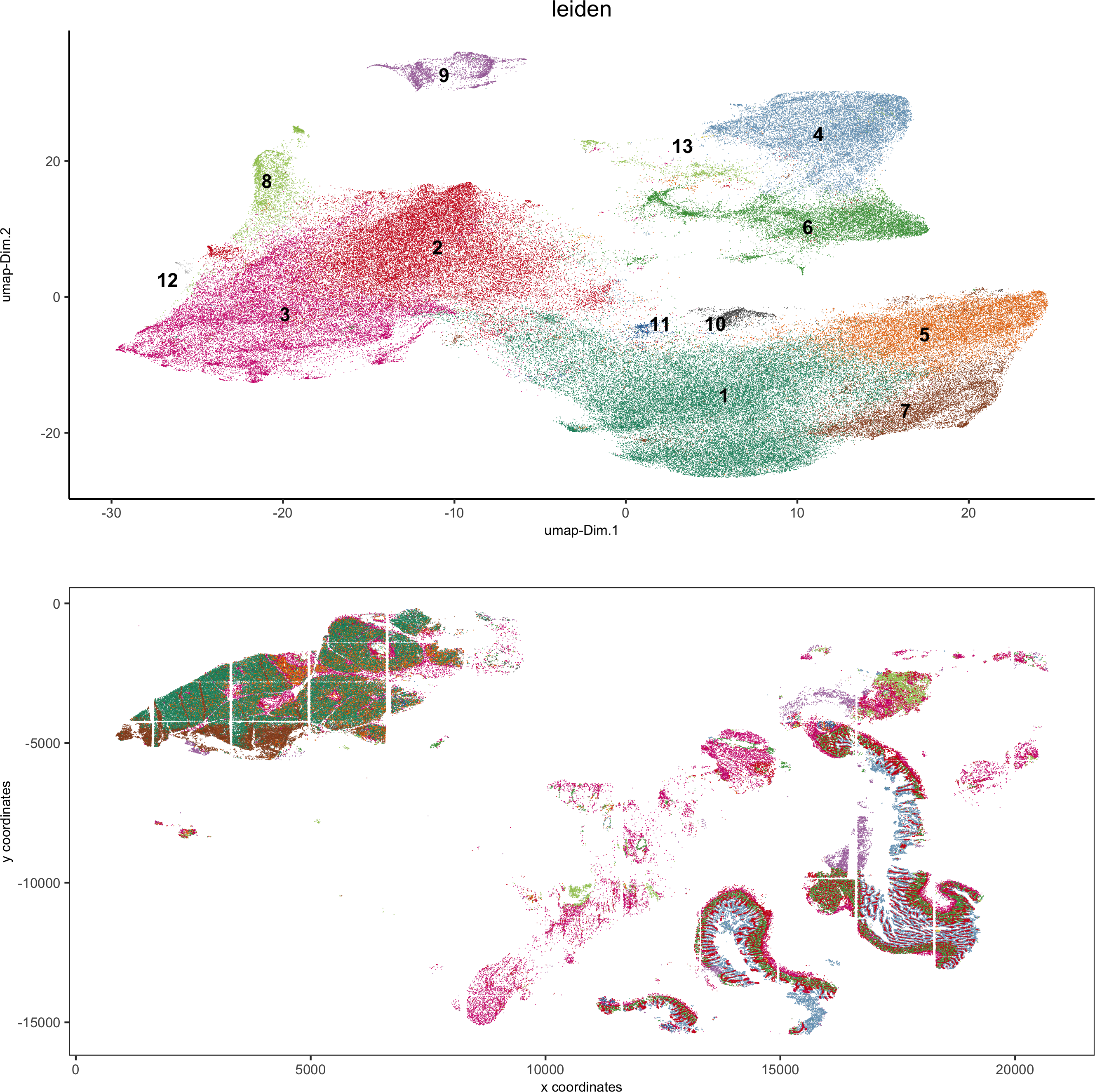
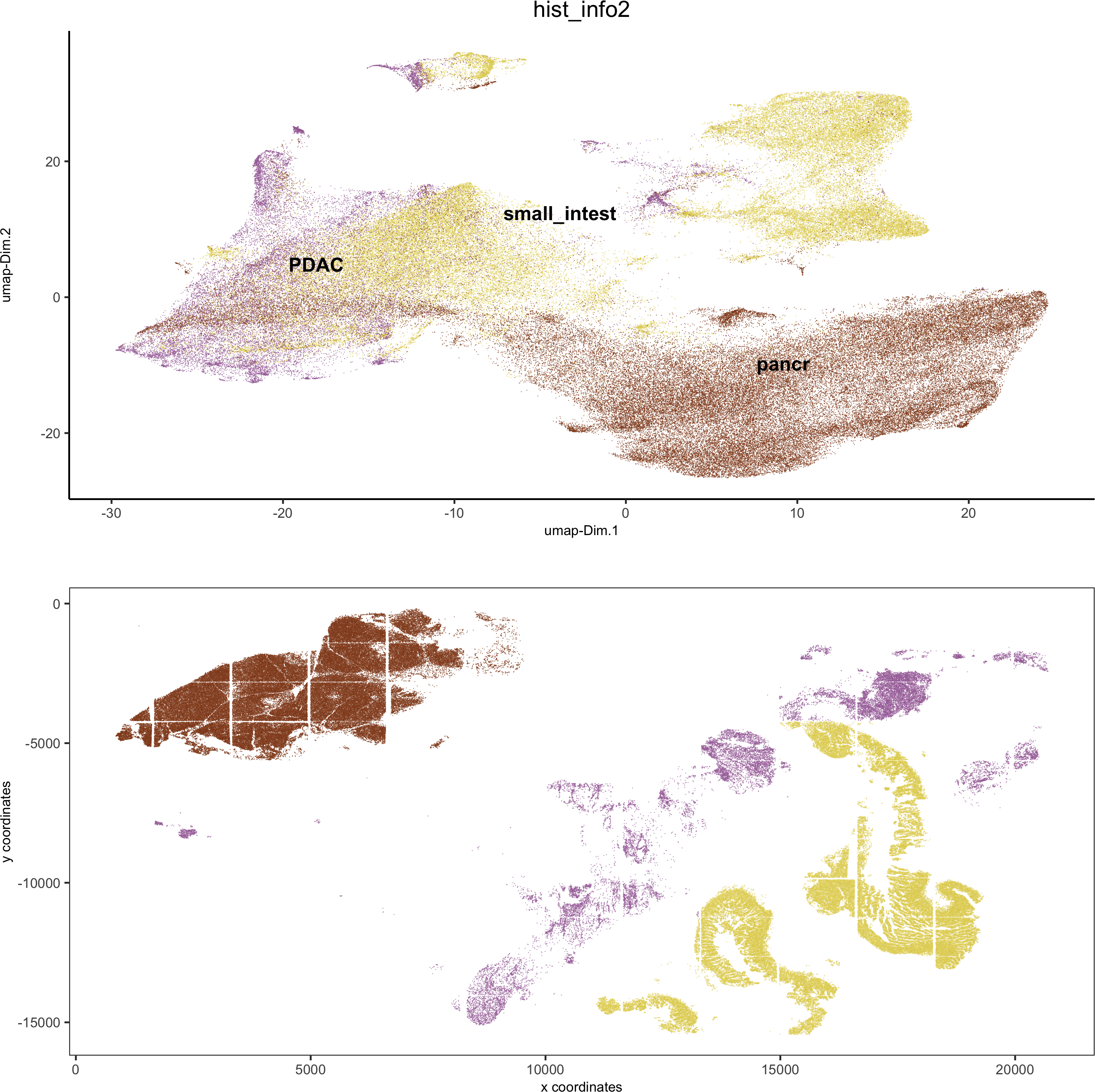
5. Visualize spatial and expression space

spatDimPlot2D(gobject = pdac_test, cell_color = 'leiden',spat_point_shape = 'no_border', spat_point_size = 0.2,dim_point_shape = 'no_border', dim_point_size = 0.2,cell_color_code = leiden_colors,save_param = list(save_name = '5_a_spatdimplot'))

spatDimPlot2D(gobject = pdac_test, cell_color = 'leiden',spat_point_shape = 'border',spat_point_size = 0.2, spat_point_border_stroke = 0.01,dim_point_shape = 'border', dim_point_size = 0.2,dim_point_border_stroke = 0.01, cell_color_code = leiden_colors,save_param = list(save_name = '5_b_spatdimplot'))

spatDimPlot2D(gobject = pdac_test, cell_color = 'hist_info2',spat_point_shape = 'border', spat_point_size = 0.2,spat_point_border_stroke = 0.01, dim_point_shape = 'border',dim_point_size = 0.2, dim_point_border_stroke = 0.01,save_param = list(save_name = '5_c_spatdimplot'))

6. Cell type marker gene detection

# resolution 0.2
cluster_column = 'leiden'
# gini
markers_gini = findMarkers_one_vs_all(gobject = pdac_test,method = "gini",expression_values = "scaled",cluster_column = cluster_column,min_genes = 5)
markergenes_gini = unique(markers_gini[, head(.SD, 5), by = "cluster"][["genes"]])
plotMetaDataHeatmap(pdac_test, expression_values = "norm",metadata_cols = c(cluster_column),selected_genes = markergenes_gini, 
custom_cluster_order = c(1, 10, 3, 12, 8, 2, 9, 6, 11, 13, 4, 5, 7),y_text_size = 8, show_values = 'zscores_rescaled',save_param = list(save_name = '6_a_metaheatmap'))

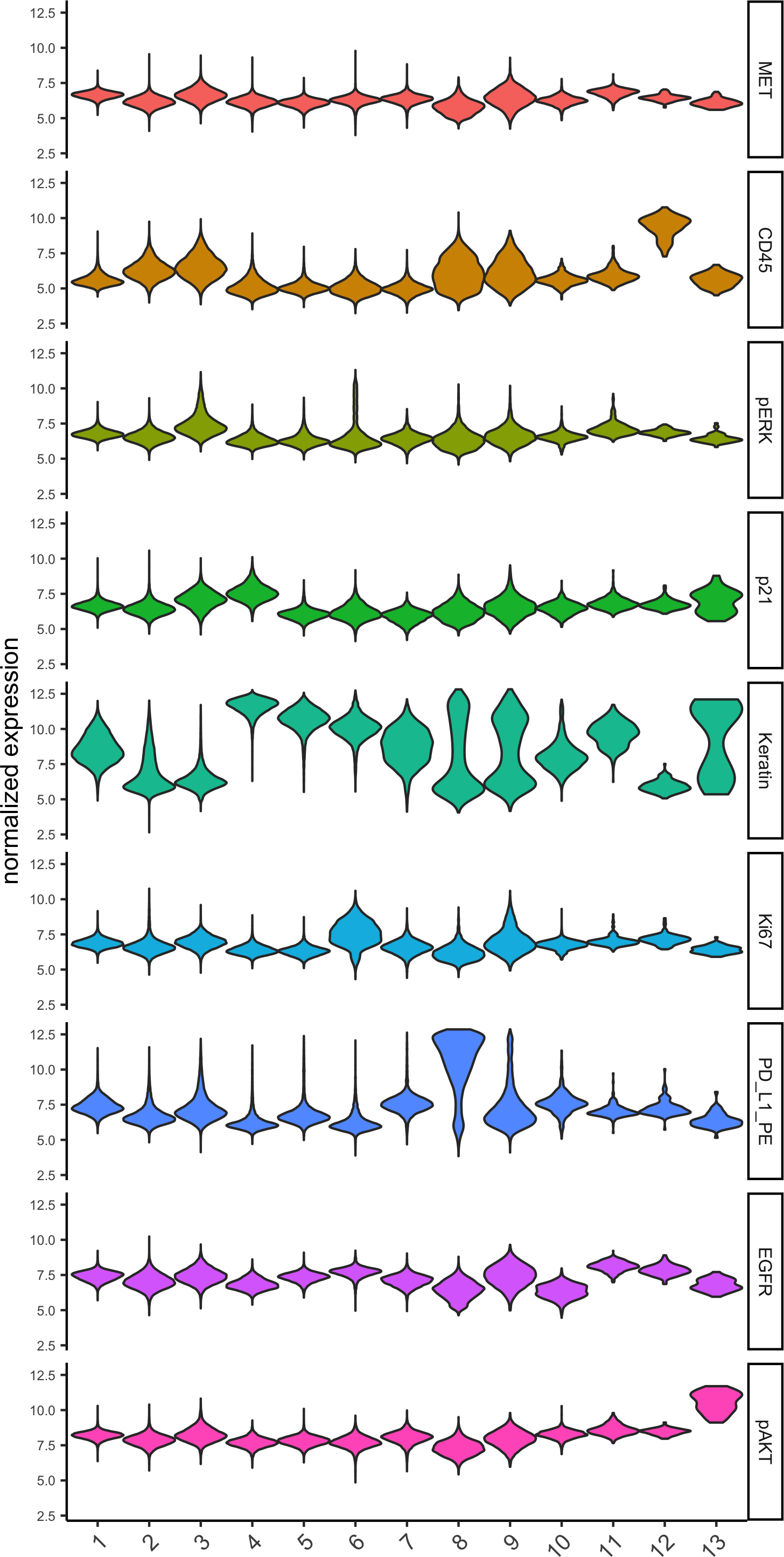
topgenes_gini = markers_gini[, head(.SD, 1), by = 'cluster']$genes
violinPlot(pdac_test, genes = unique(topgenes_gini), cluster_column = cluster_column,strip_text = 8, strip_position = 'right',save_param = c(save_name = '6_b_violinplot_gini', base_width = 5, base_height = 10))

7. Cell type annotation

Metadata heatmap

Inspect the potential cell type markers

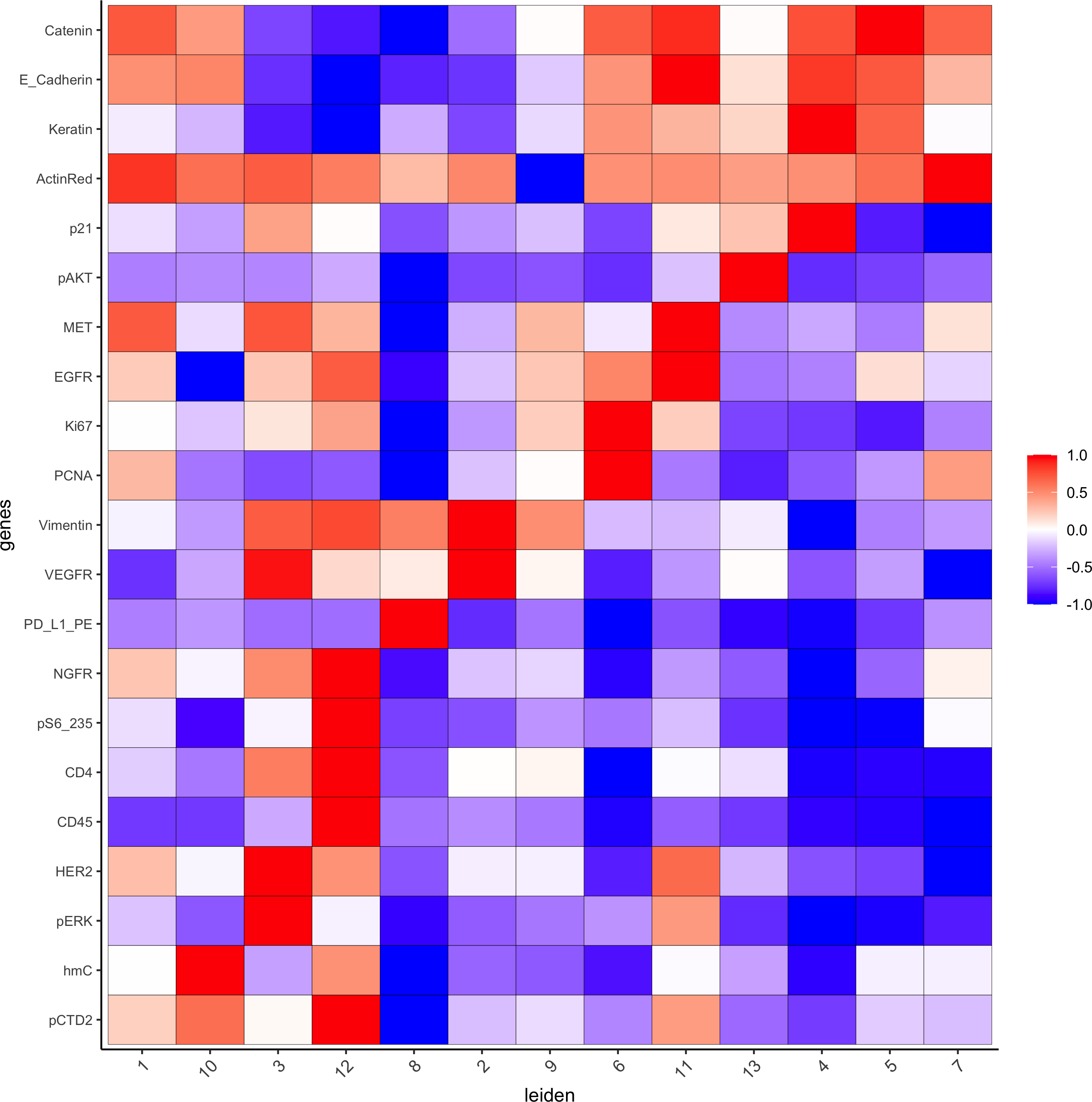
## all genes heatmap
plotMetaDataHeatmap(pdac_test, expression_values = "norm", metadata_cols = 'leiden', 
custom_cluster_order = c(1, 10, 3, 12, 8, 2, 9, 6, 11, 13, 4, 5, 7),y_text_size = 8, show_values = 'zscores_rescaled',save_param = list(save_name = '7_a_metaheatmap'))

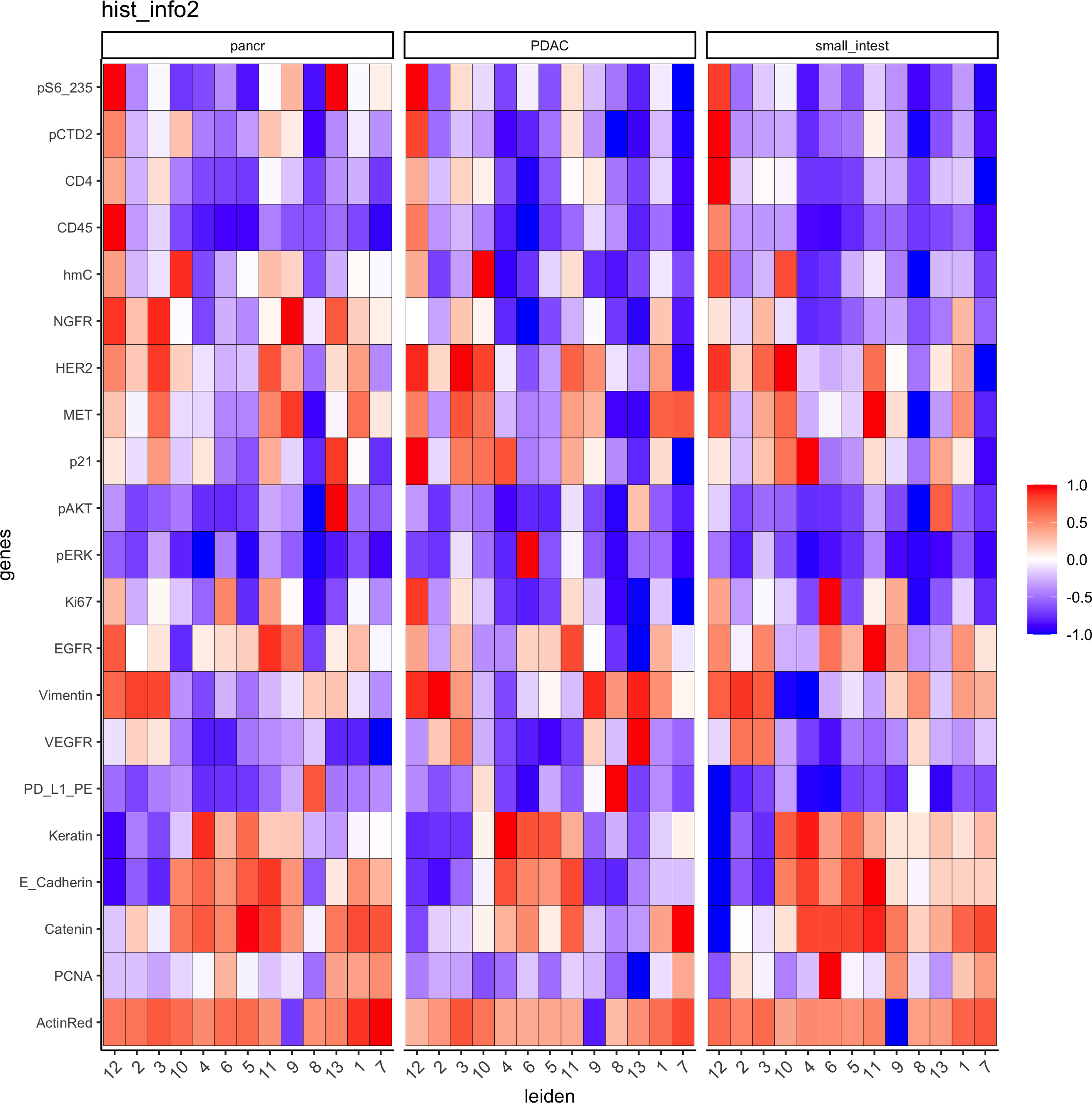
Inspect the potential cell type markers stratified by tissue location

plotMetaDataHeatmap(pdac_test, expression_values = "norm", metadata_cols = c('leiden','hist_info2'), 
first_meta_col = 'leiden', second_meta_col = 'hist_info2',y_text_size = 8, show_values = 'zscores_rescaled',save_param = list(save_name = '7_b_metaheatmap'))

Spatial subsets

Inspect subsets of the data based on tissue location

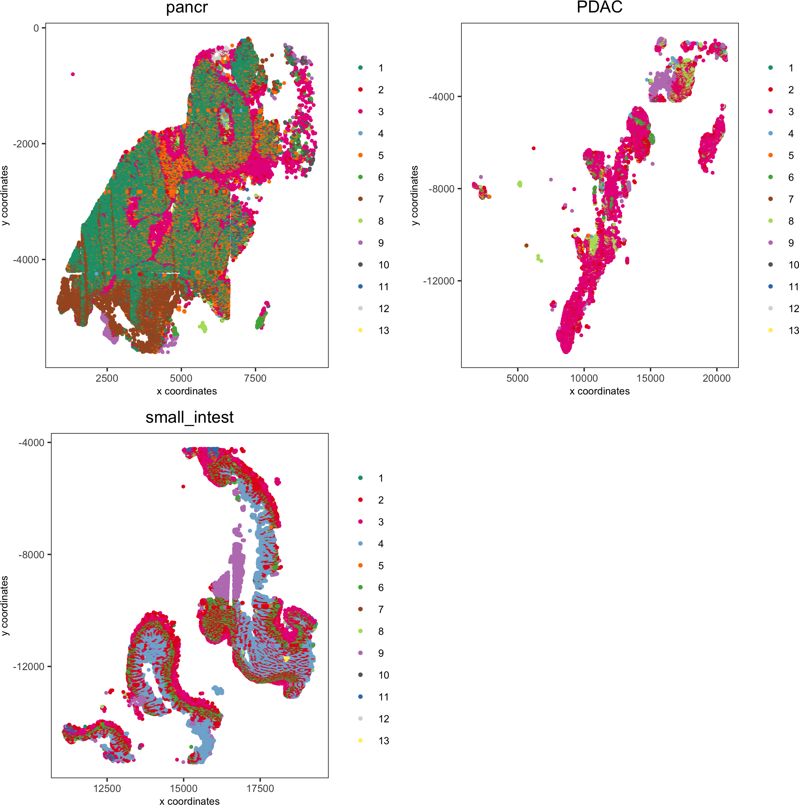
spatPlot(pdac_test, cell_color = 'leiden', cell_color_code = leiden_colors,point_shape = 'no_border', point_size = 0.75, group_by = 'hist_info2',save_param = list(save_name = '7_c_spatplot'))

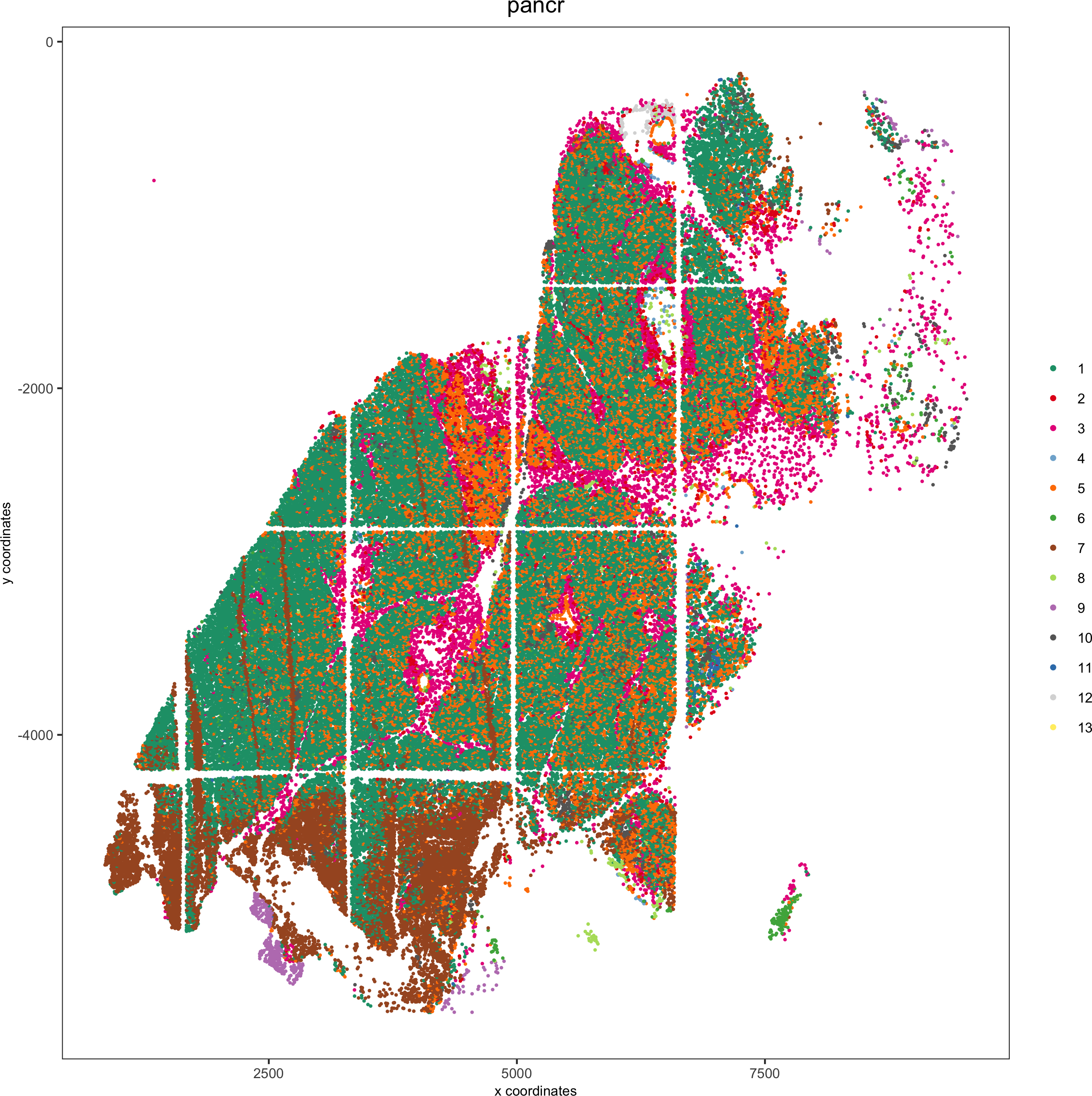
spatPlot(pdac_test, cell_color = 'leiden', cell_color_code = leiden_colors,point_shape = 'no_border', point_size = 0.3,group_by = 'hist_info2', group_by_subset = c('pancr'), cow_n_col = 1,save_param = list(save_name = '7_d_spatplot'))

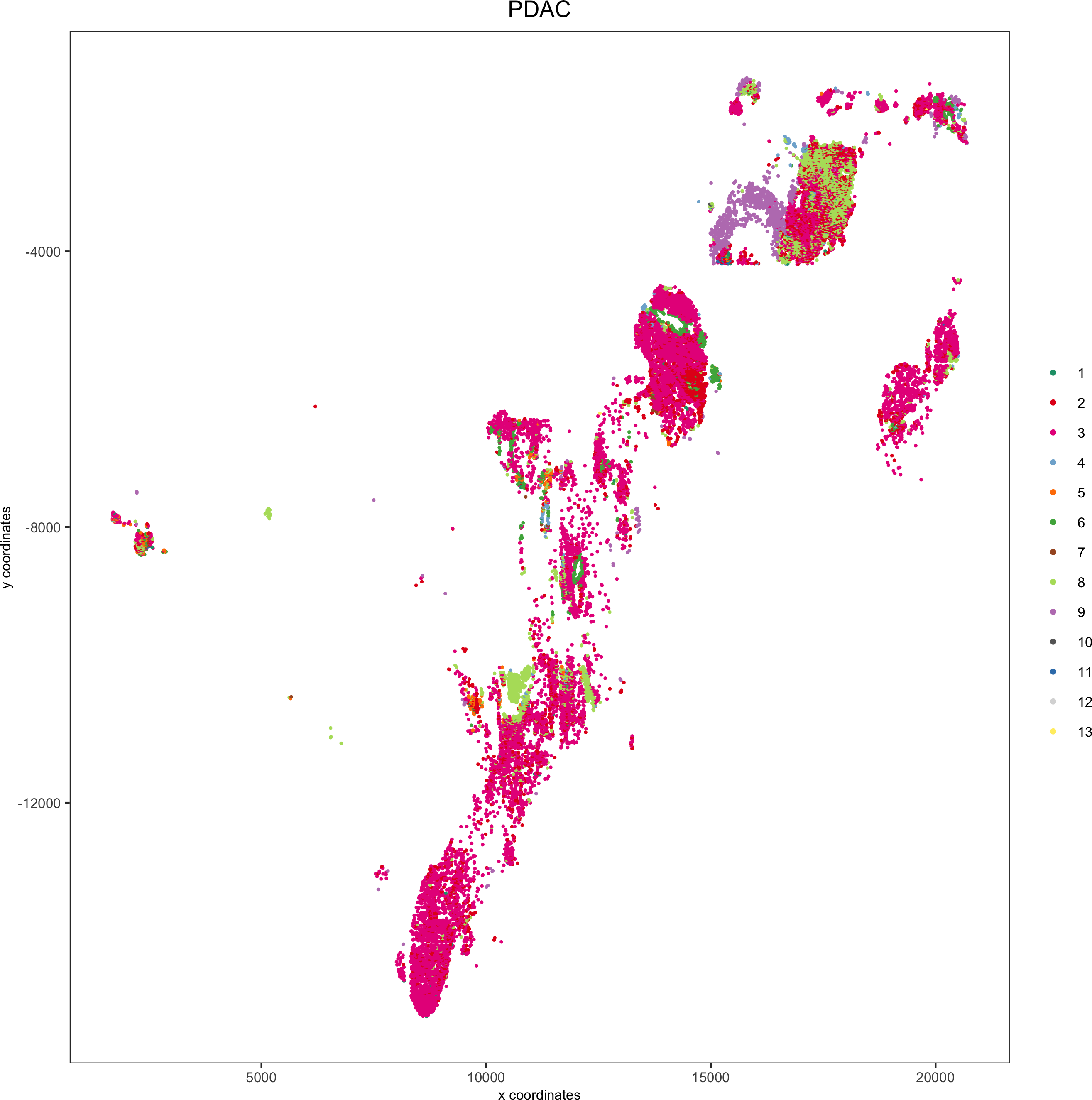
spatPlot(pdac_test, cell_color = 'leiden', cell_color_code = leiden_colors,point_shape = 'no_border', point_size = 0.3,group_by = 'hist_info2', group_by_subset = c('PDAC'), cow_n_col = 1,save_param = list(save_name = '7_e_spatplot'))

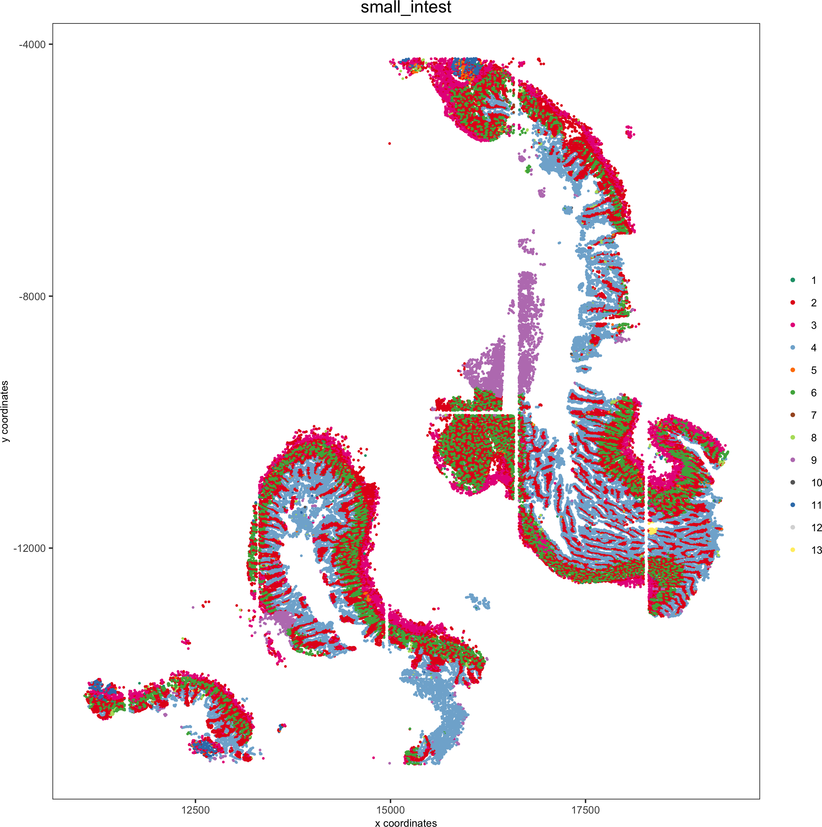
spatPlot(pdac_test, cell_color = 'leiden', cell_color_code = leiden_colors,point_shape = 'no_border', point_size = 0.3,group_by = 'hist_info2', group_by_subset = c('small_intest'), cow_n_col = 1,save_param = list(save_name = '7_f_spatplot'))

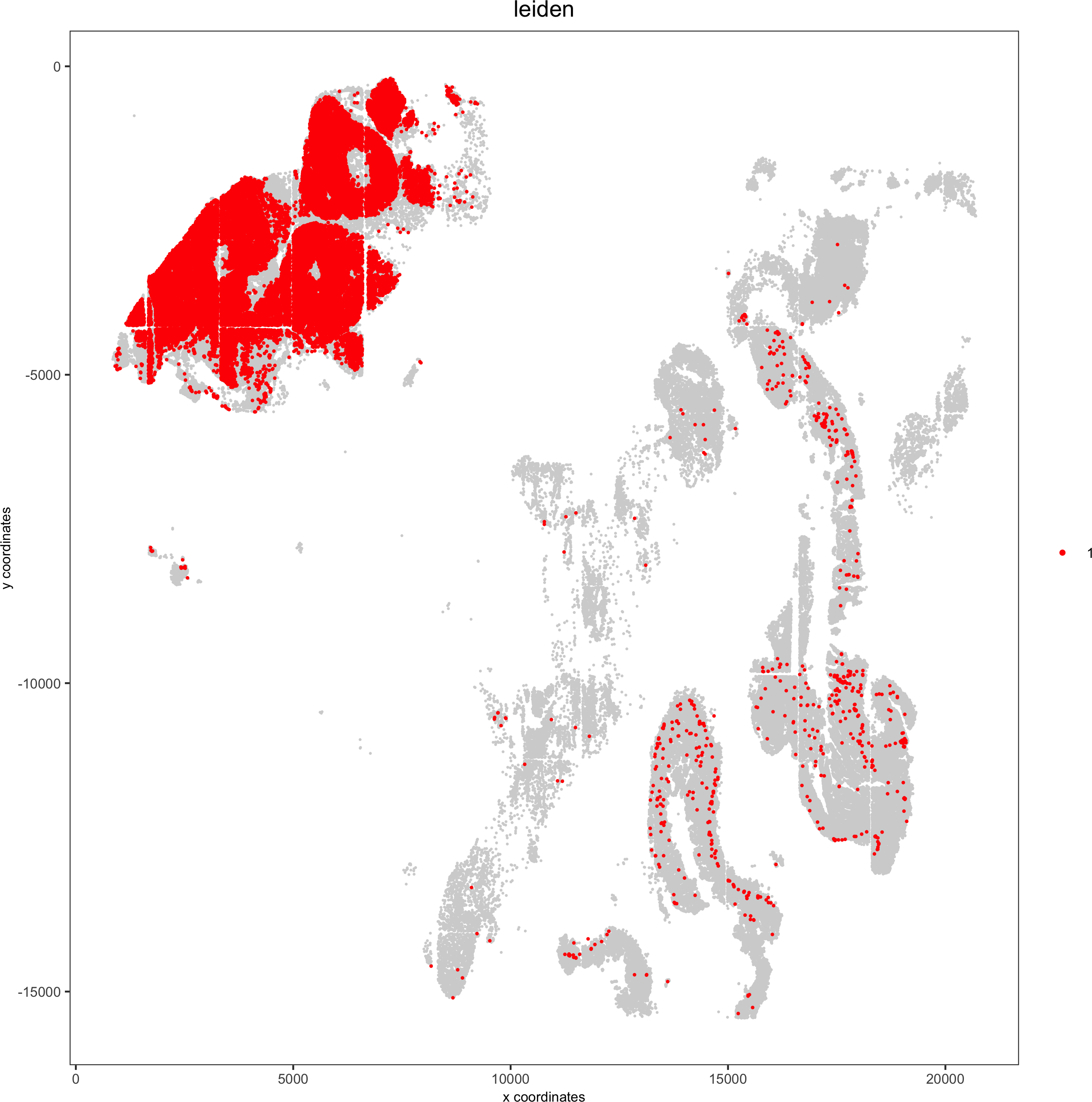
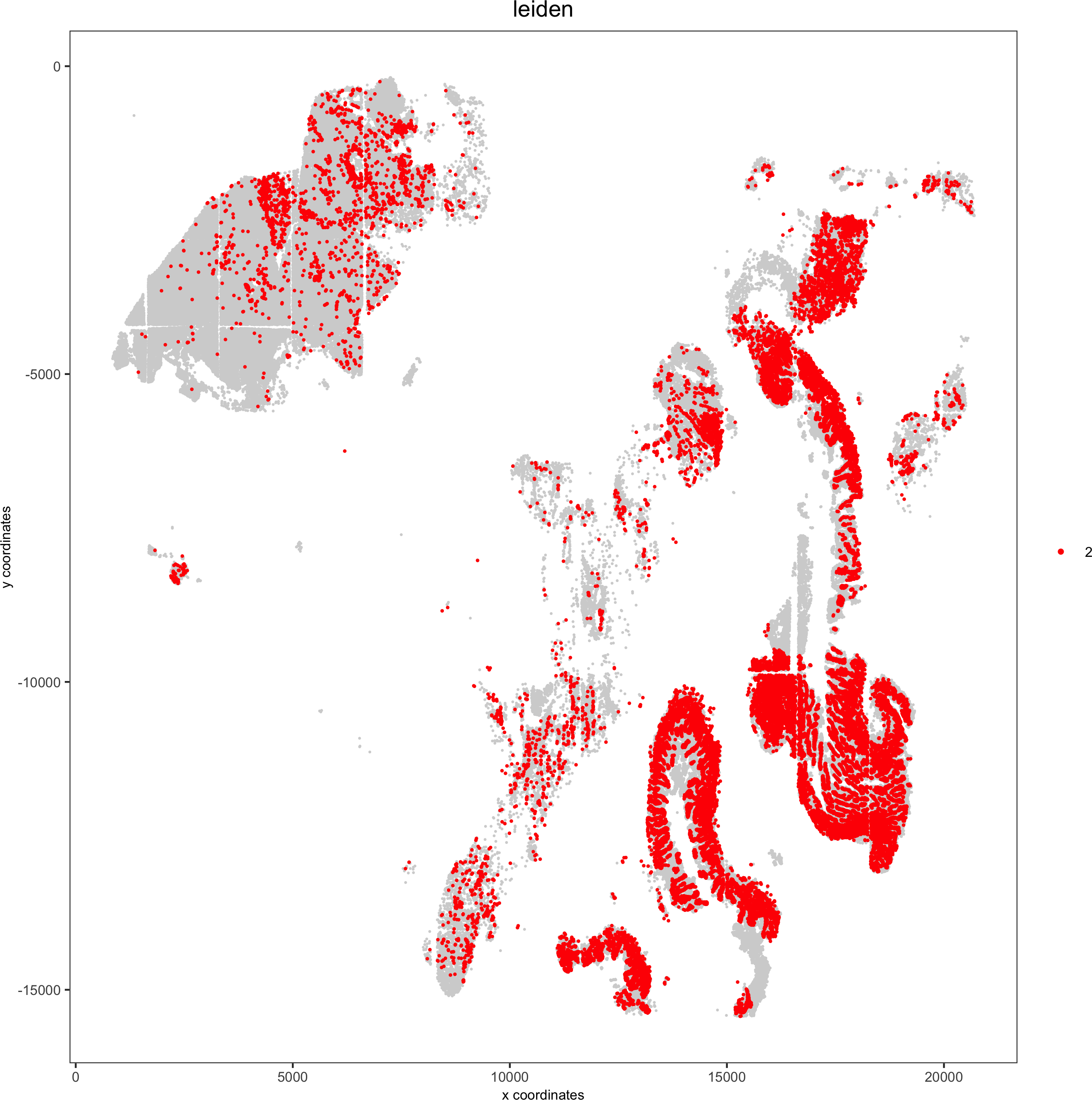
Spatial distribution of clusters

Visually inspect the spatial distribution of different clusters

# spatial enrichment of groups
for(group in unique(pDataDT(pdac_test)$leiden)) {
spatPlot(pdac_test, cell_color = 'leiden', point_shape = 'no_border',point_size = 0.3, other_point_size = 0.1,select_cell_groups = group, cell_color_code = 'red',save_param = list(save_name = paste0('7_g_spatplot_', group)))
}

Here we show a subset of the resulting plots:

Annotate clusters based on spatial position and dominant expression patterns

cell_metadata =  pDataDT(pdac_test)
cluster_data = cell_metadata[, .N, by = c('leiden', 'hist_info2')]
cluster_data[, fraction:= round(N/sum(N), 2), by = c('leiden')]
data.table::setorder(cluster_data, leiden, hist_info2, fraction)
# final annotation
names = 1:13
location = c('pancr', 'intest', 'general', 'intest', 'pancr','intest', 'pancr', 'canc', 'general', 'pancr','general', 'pancr', 'intest')
feats = c('epithelial_I', 'fibroblast_VEGFR+', 'stroma_HER2+_pERK+', 'epithelial_lining_p21+', 'epithelial_keratin','epithelial_prolif', 'epithelial_actin++', 'immune_PD-L1+', 'stromal_actin-', 'epithelial_tx_active','epithelial_MET+_EGFR+', 'immune_CD45+', 'epithelial_pAKT')
annot_dt = data.table::data.table('names' = names, 'location' = location, 'feats' = feats)
annot_dt[, annotname := paste0(location,'_',feats)]
cell_annot = annot_dt$annotname;names(cell_annot) = annot_dt$names
pdac_test = annotateGiotto(pdac_test, annotation_vector = cell_annot, cluster_column = 'leiden')
# specify colors
leiden_colors
leiden_names = annot_dt$annotname; names(leiden_names) = annot_dt$names
cell_annot_colors = leiden_colors
names(cell_annot_colors) = leiden_names[names(leiden_colors)]
# covisual
spatDimPlot(gobject = pdac_test, cell_color = 'cell_types', cell_color_code = cell_annot_colors,spat_point_shape = 'border', spat_point_size = 0.2, spat_point_border_stroke = 0.01,dim_point_shape = 'border', dim_point_size = 0.2, dim_point_border_stroke = 0.01,dim_show_center_label = F, spat_show_legend = T, dim_show_legend = T, legend_symbol_size = 3,save_param = list(save_name = '7_h_spatdimplot'))

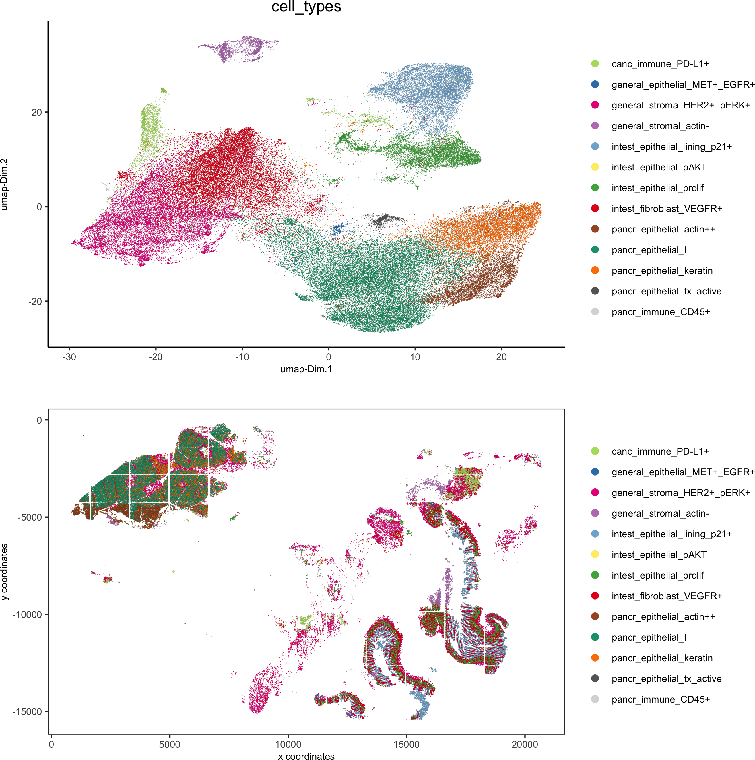
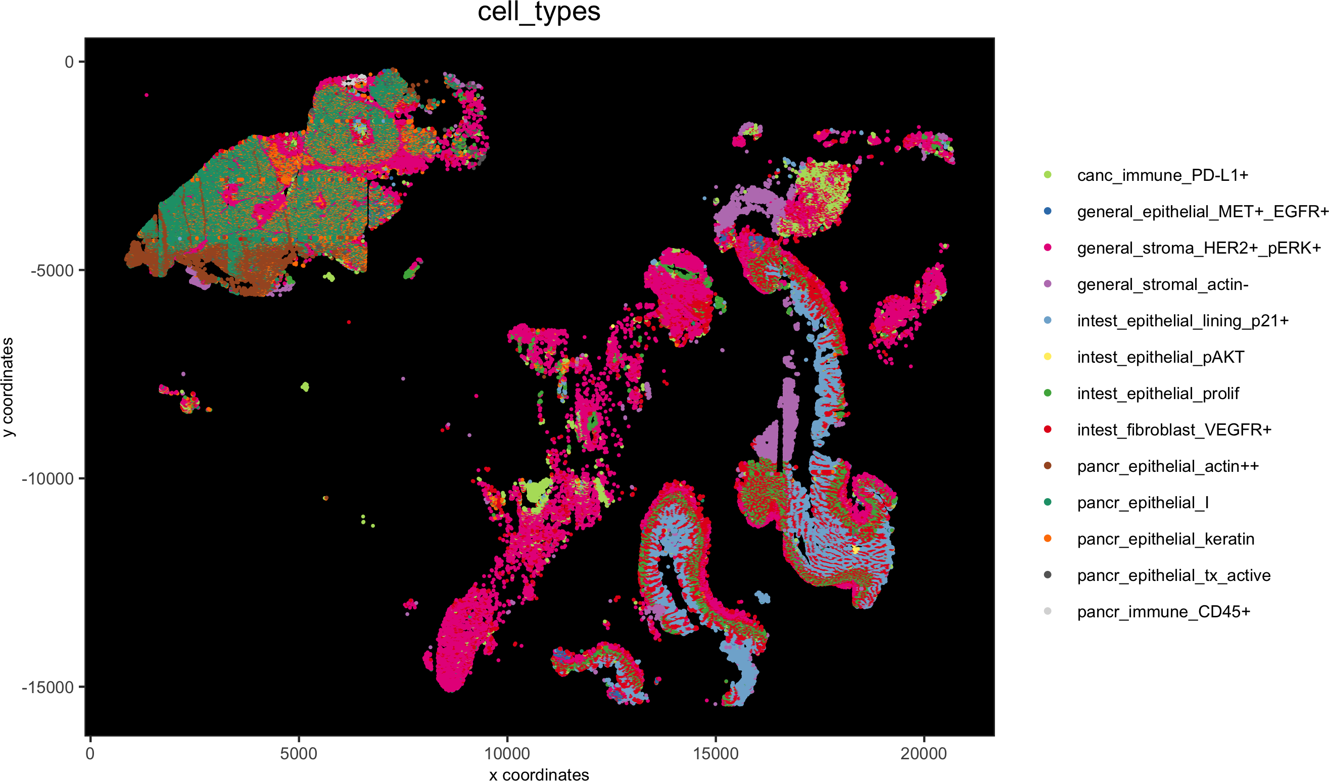
# spatial only
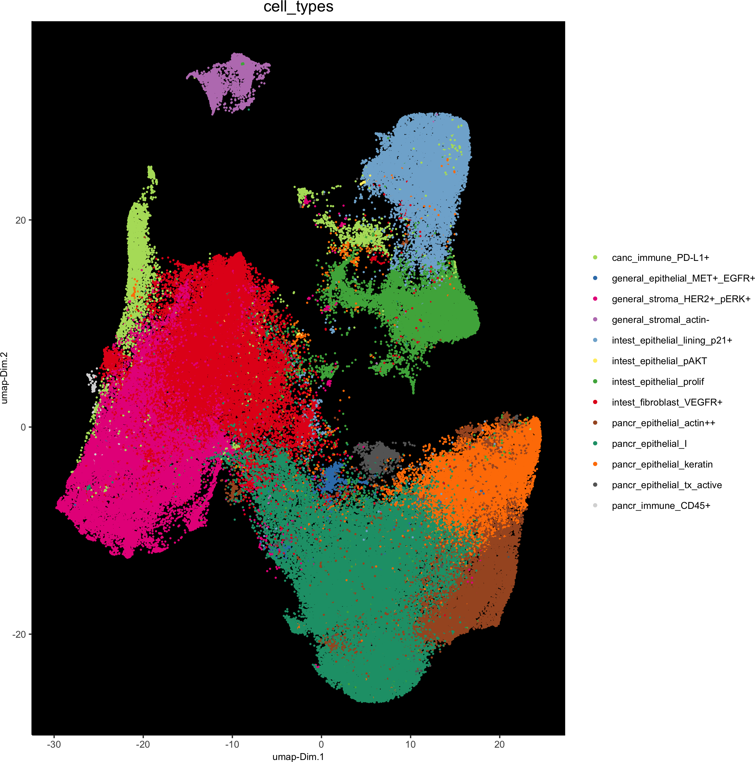
spatPlot(gobject = pdac_test, cell_color = 'cell_types', point_shape = 'no_border', point_size = 0.2, 
coord_fix_ratio = 1, show_legend = T, cell_color_code = cell_annot_colors, background_color = 'black',save_param = list(save_name = '7_i_spatplot'))

# dimension only
plotUMAP(gobject = pdac_test, cell_color = 'cell_types', point_shape = 'no_border', point_size = 0.2, 
show_legend = T, cell_color_code = cell_annot_colors, show_center_label = F, background_color = 'black',save_param = list(save_name = '7_j_umap'))

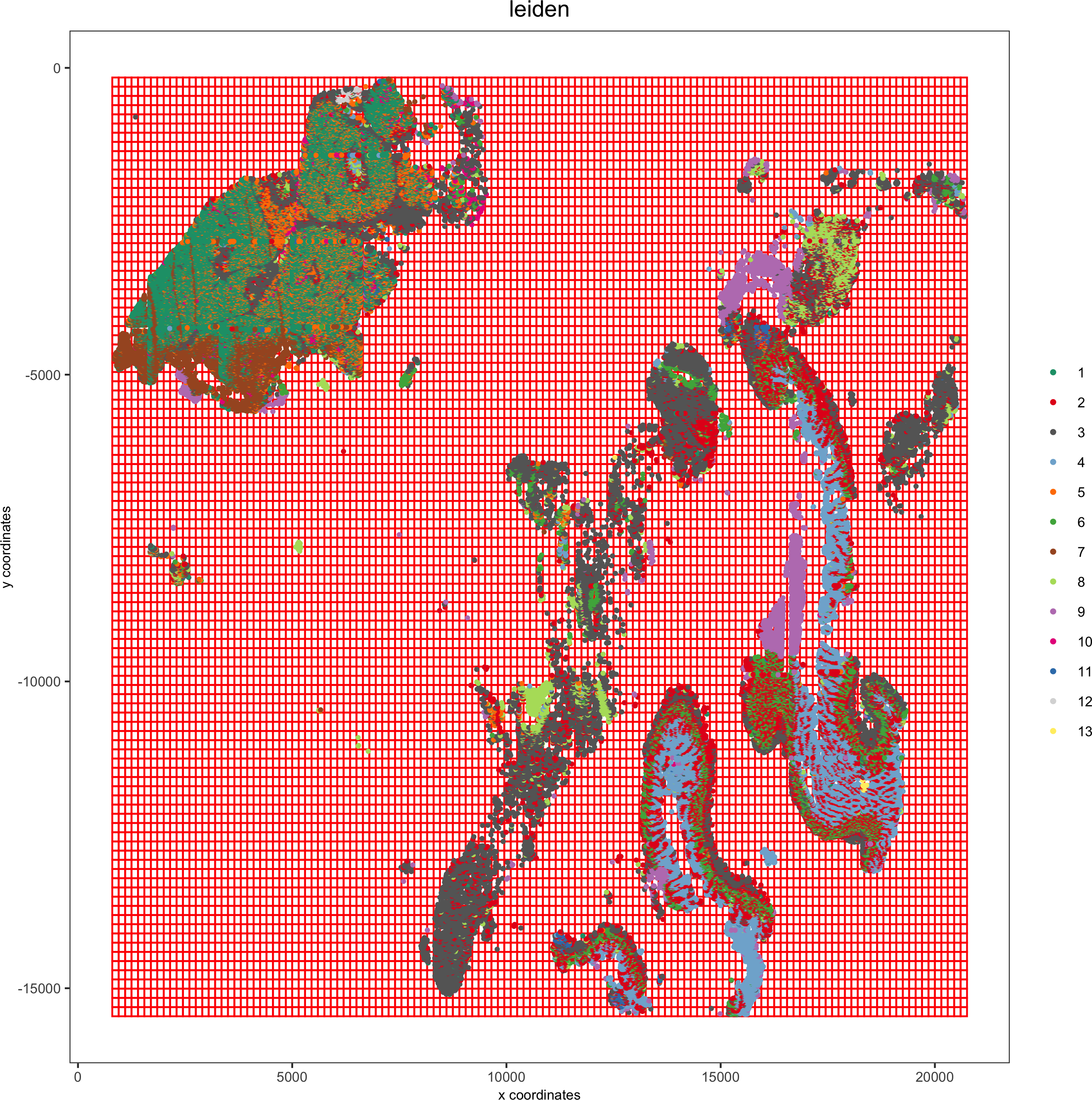
8. Spatial grid

pdac_test <- createSpatialGrid(gobject = pdac_test,sdimx_stepsize = 150,sdimy_stepsize = 150,minimum_padding = 0)
spatPlot(pdac_test, 
cell_color = 'leiden', 
show_grid = T, point_size = 0.75, point_shape = 'no_border',grid_color = 'red', spatial_grid_name = 'spatial_grid',save_param = list(save_name = '8_a_spatplot'))

9. Spatial network

pdac_test <- createSpatialNetwork(gobject = pdac_test, minimum_k = 2)

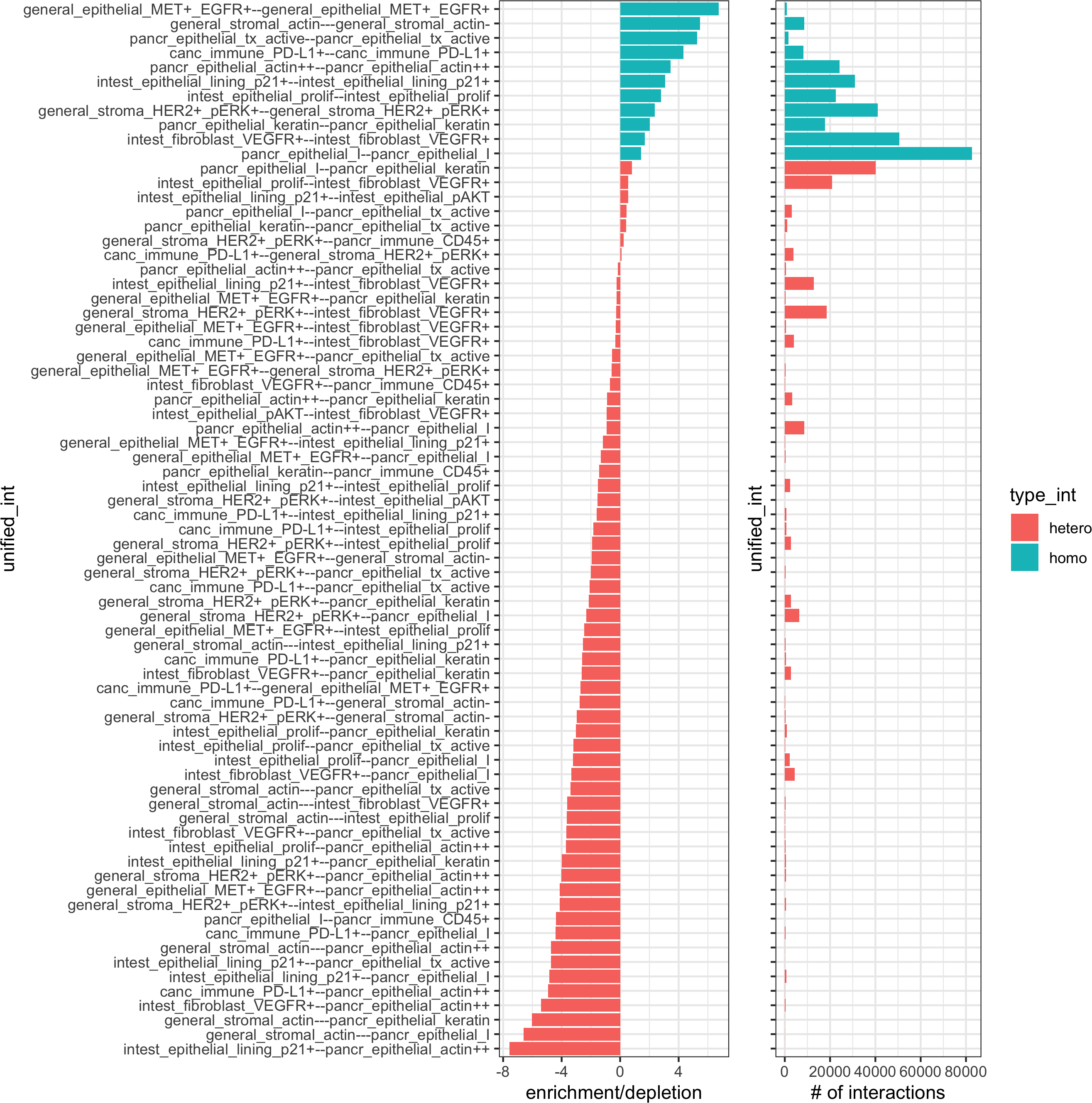
10. Cell-cell preferential proximity

## calculate frequently seen proximities
cell_proximities = cellProximityEnrichment(gobject = pdac_test,cluster_column = 'cell_types',spatial_network_name = 'Delaunay_network',number_of_simulations = 200)
## barplot
cellProximityBarplot(gobject = pdac_test, CPscore = cell_proximities, min_orig_ints = 5, min_sim_ints = 5,save_param = list(save_name = '12_a_barplot'))

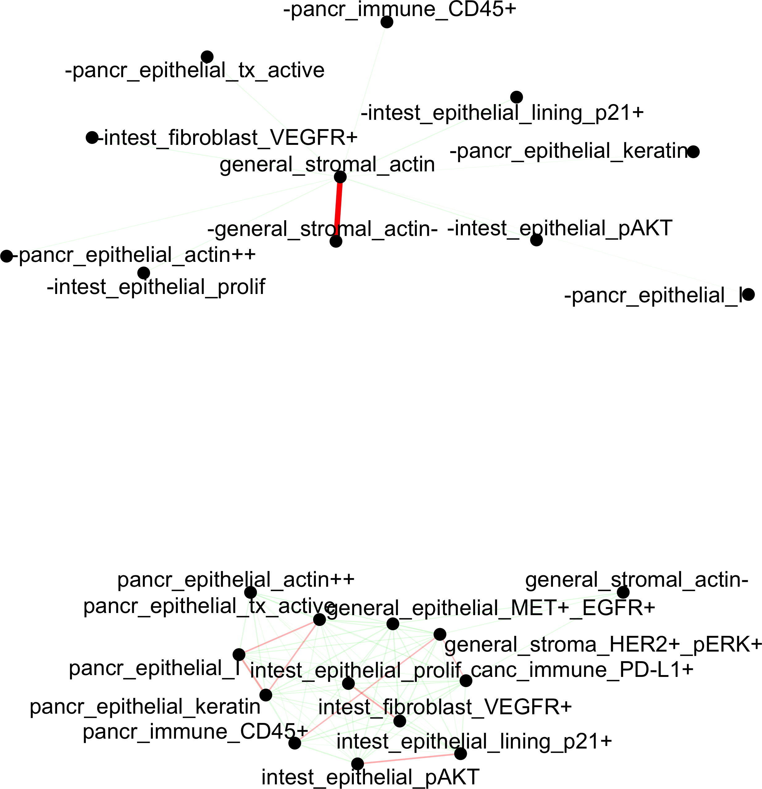
## network
cellProximityNetwork(gobject = pdac_test, CPscore = cell_proximities,remove_self_edges = T, only_show_enrichment_edges = F,save_param = list(save_name = '12_b_network'))

## visualization
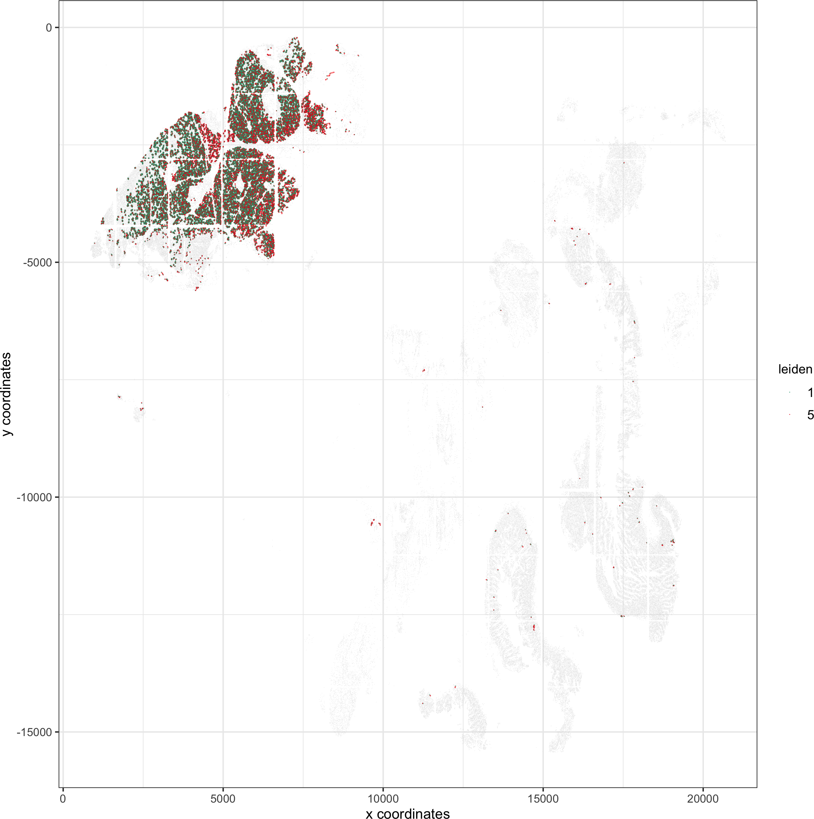
spec_interaction = "1--5"
cellProximitySpatPlot2D(gobject = pdac_test, point_select_border_stroke = 0,interaction_name = spec_interaction,cluster_column = 'leiden', show_network = T,cell_color = 'leiden', coord_fix_ratio = NULL,point_size_select = 0.3, point_size_other = 0.1,save_param = list(save_name = '12_c_proxspatplot'))

11. analyses for paper

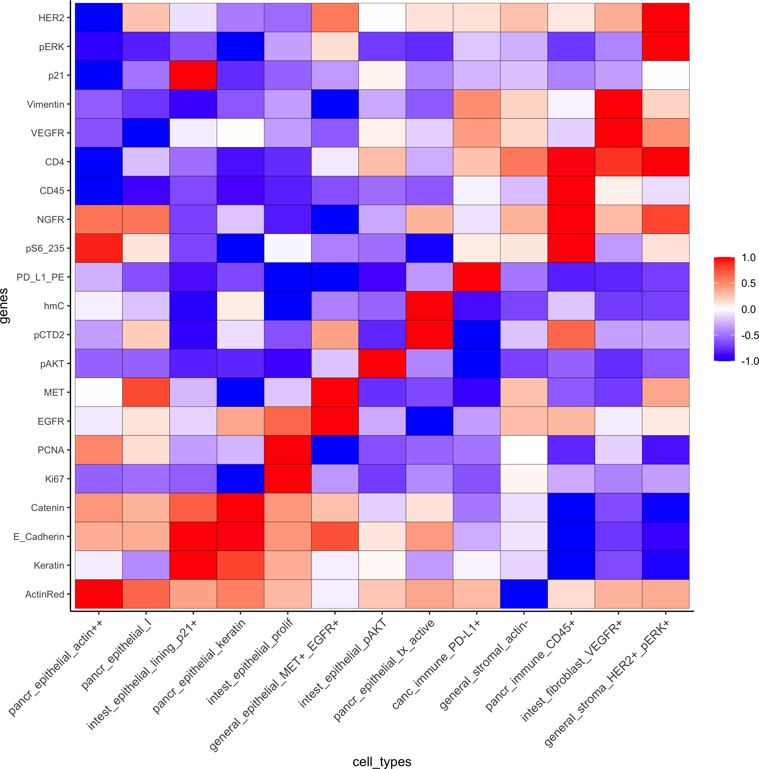
Heatmap for cell type annotation:

cell_type_order_pdac = c("pancr_epithelial_actin++", "pancr_epithelial_I","intest_epithelial_lining_p21+", "pancr_epithelial_keratin", 
"intest_epithelial_prolif" ,"general_epithelial_MET+_EGFR+","intest_epithelial_pAKT", "pancr_epithelial_tx_active","canc_immune_PD-L1+","general_stromal_actin-","pancr_immune_CD45+", "intest_fibroblast_VEGFR+","general_stroma_HER2+_pERK+")

plotMetaDataHeatmap(pdac_test, expression_values = "scaled", metadata_cols = c('cell_types'), 
custom_cluster_order = cell_type_order_pdac,y_text_size = 8, show_values = 'zscores_rescaled',save_param = list(save_name = 'xx_a_metaheatmap'))

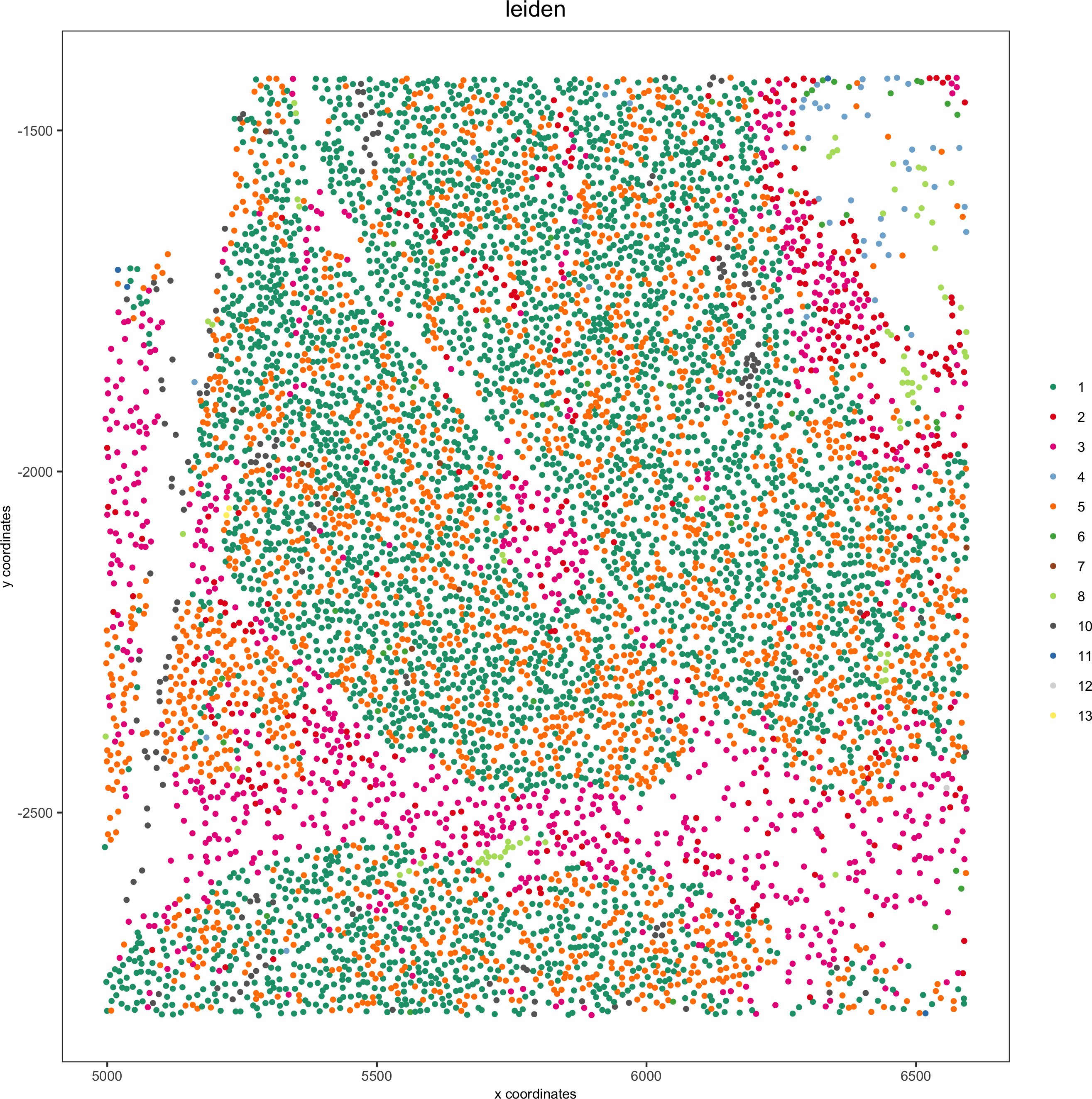
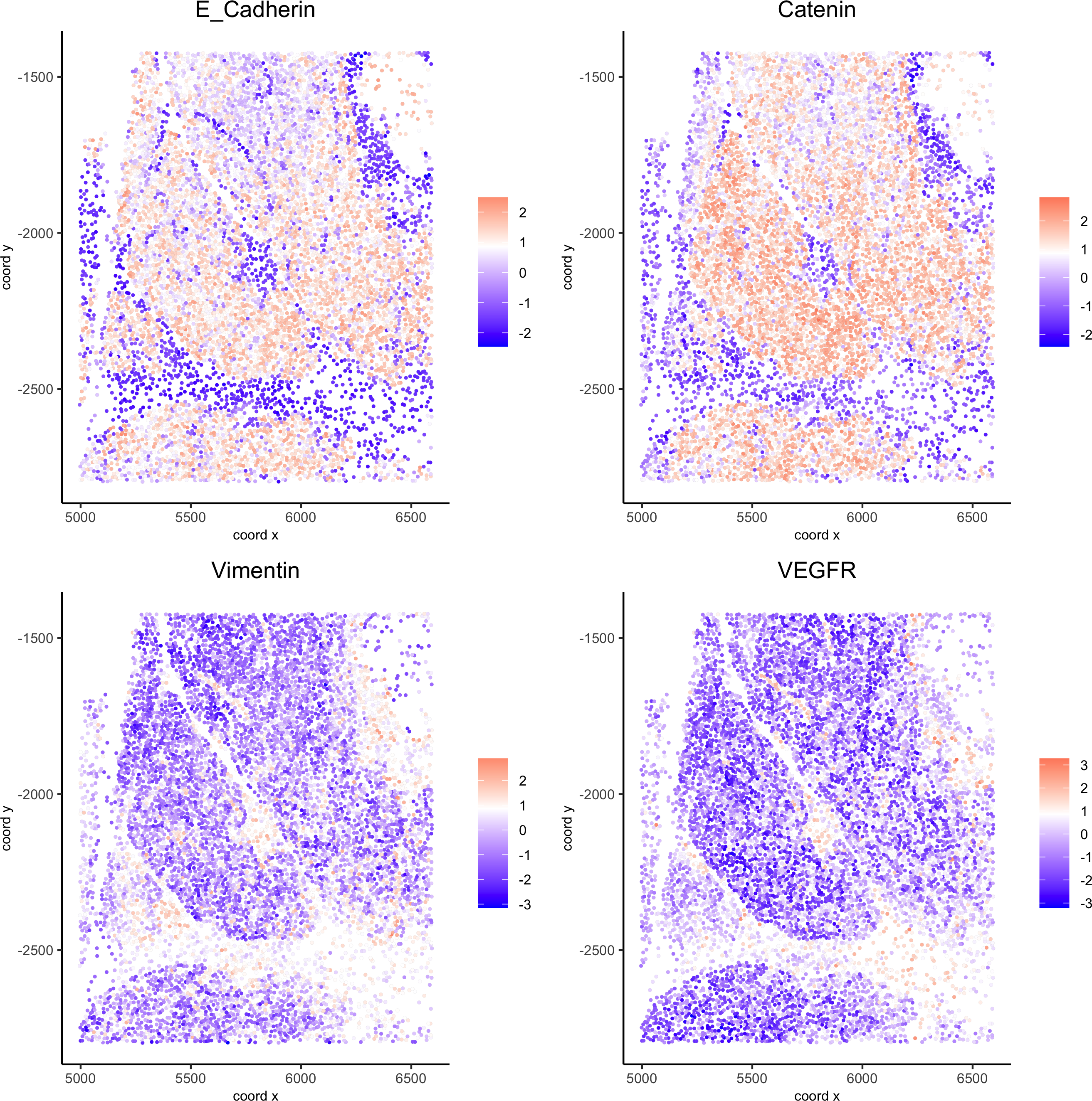
Pancreas

Highlight region in pancreas:

## pancreas region ##
my_pancreas_Ids = pdac_metadata[frame == 17][['cell_ID']]
my_pancreas_giotto = subsetGiotto(pdac_test, cell_ids = my_pancreas_Ids)

spatPlot(my_pancreas_giotto, cell_color = 'leiden', point_shape = 'no_border', 
point_size = 1, cell_color_code = leiden_colors,save_param = list(save_name = 'xx_b_spatplot'))

spatGenePlot(my_pancreas_giotto, expression_values = 'scaled', point_border_stroke = 0.01,genes = c('E_Cadherin','Catenin', 'Vimentin',  'VEGFR'), point_size = 1,save_param = list(save_name = 'xx_c_spatgeneplot'))

plotUMAP(my_pancreas_giotto, cell_color = 'leiden', point_shape = 'no_border', point_size = 0.5, 
cell_color_code = leiden_colors, show_center_label = F,save_param = list(save_name = 'xx_d_umap'))

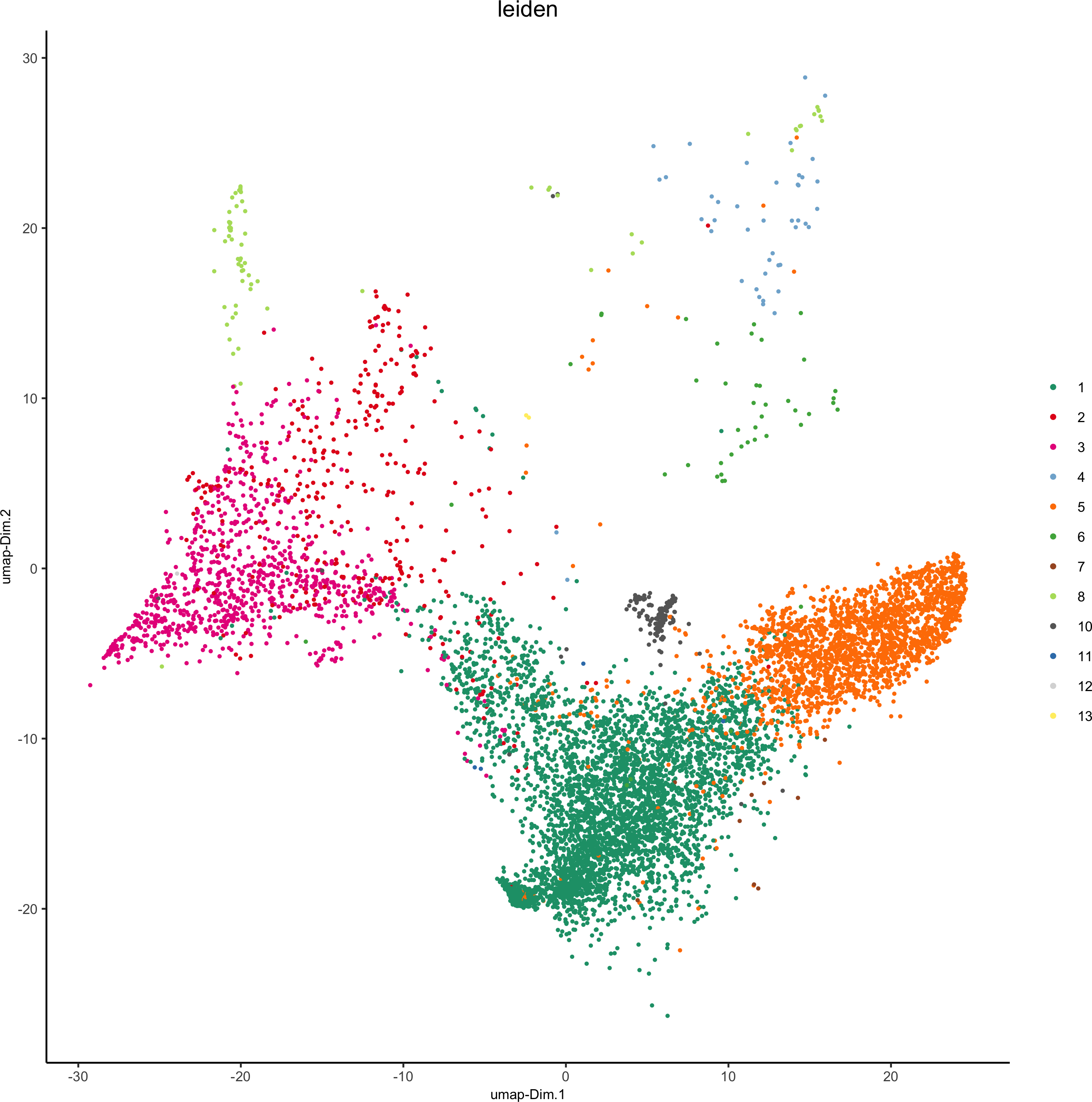
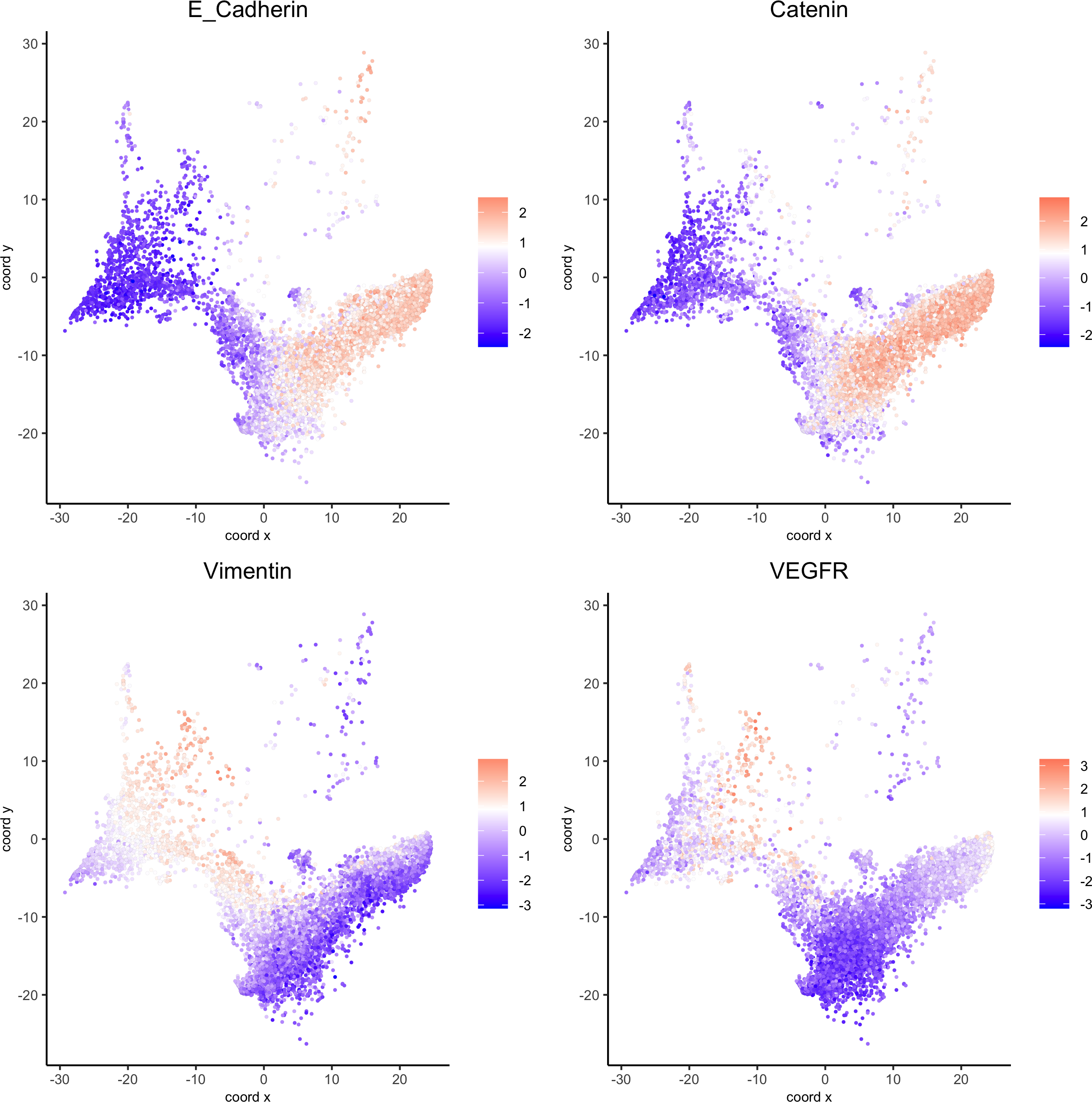
dimGenePlot(my_pancreas_giotto, expression_values = 'scaled', point_border_stroke = 0.01,genes = c('E_Cadherin','Catenin', 'Vimentin',  'VEGFR'), point_size = 1,save_param = list(save_name = 'xx_e_dimGeneplot'))

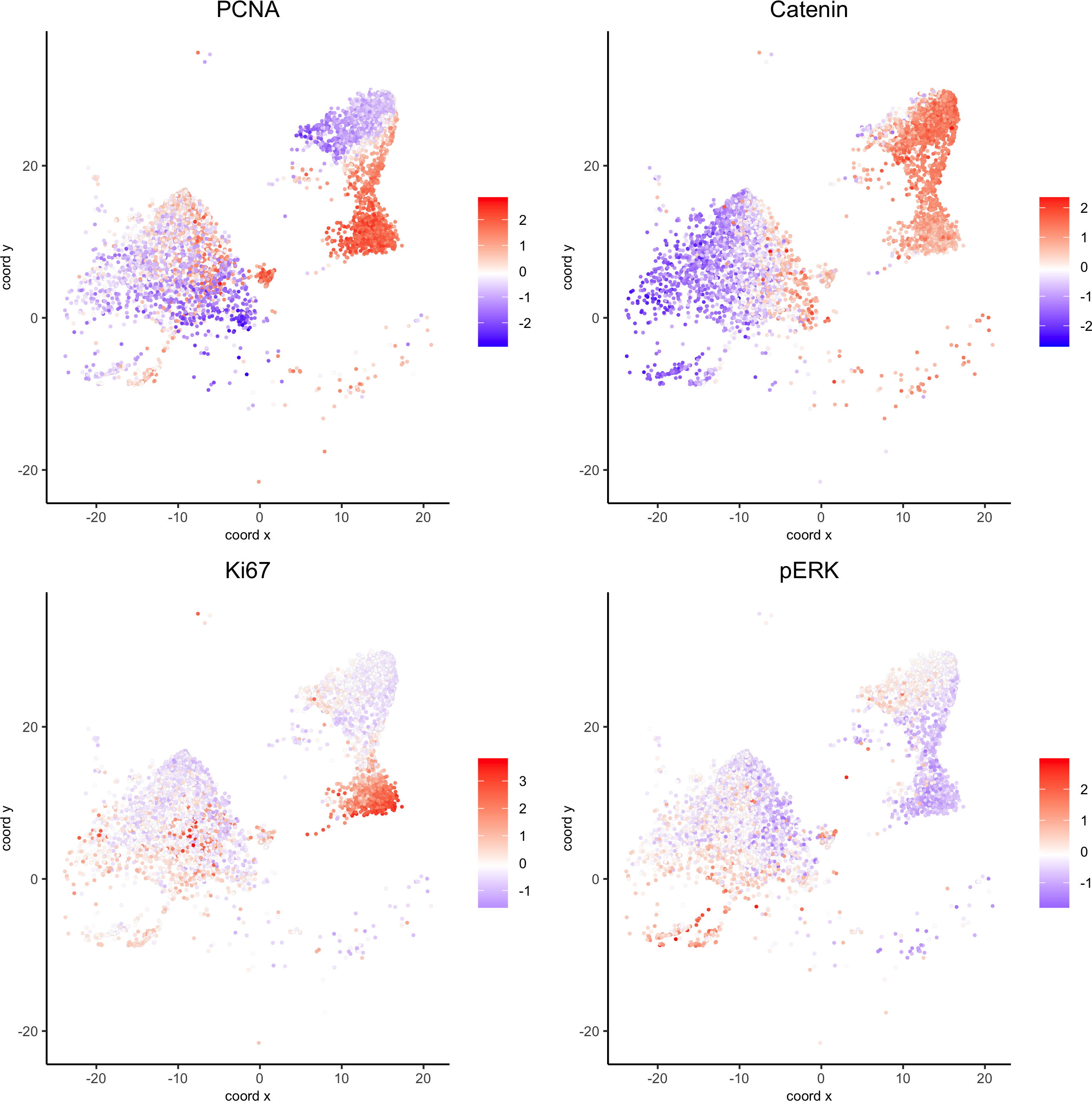
Small intestines

Highlight region in small intestines (same as in original paper):

## intestine region ##
my_intest_Ids = pdac_metadata[frame == 115][['cell_ID']]
my_intest_giotto = subsetGiotto(pdac_test, cell_ids = my_intest_Ids)
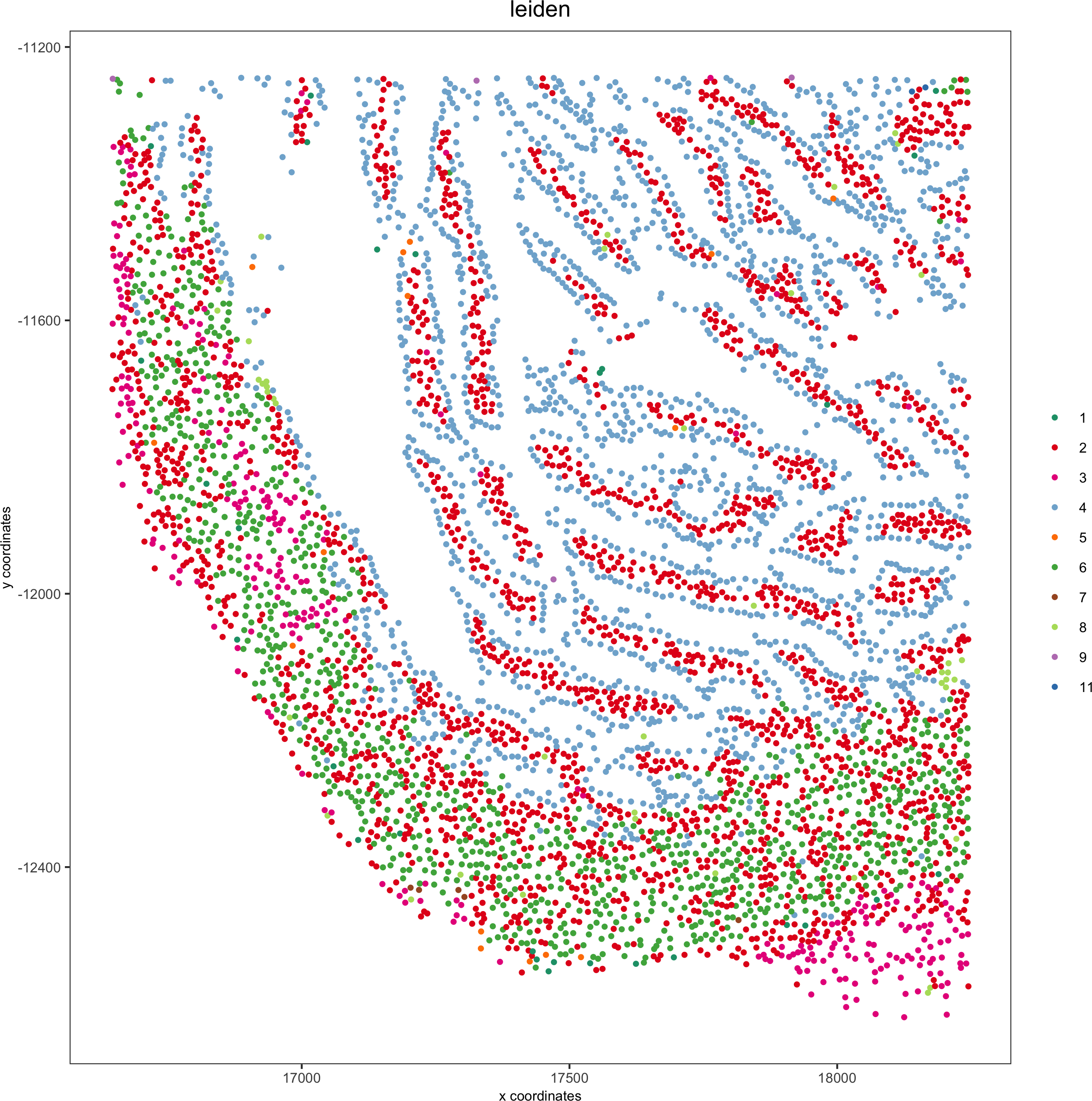
spatPlot(my_intest_giotto, cell_color = 'leiden', point_shape = 'no_border',point_size = 1, cell_color_code = leiden_colors,save_param = list(save_name = 'xx_f_spatplot'))

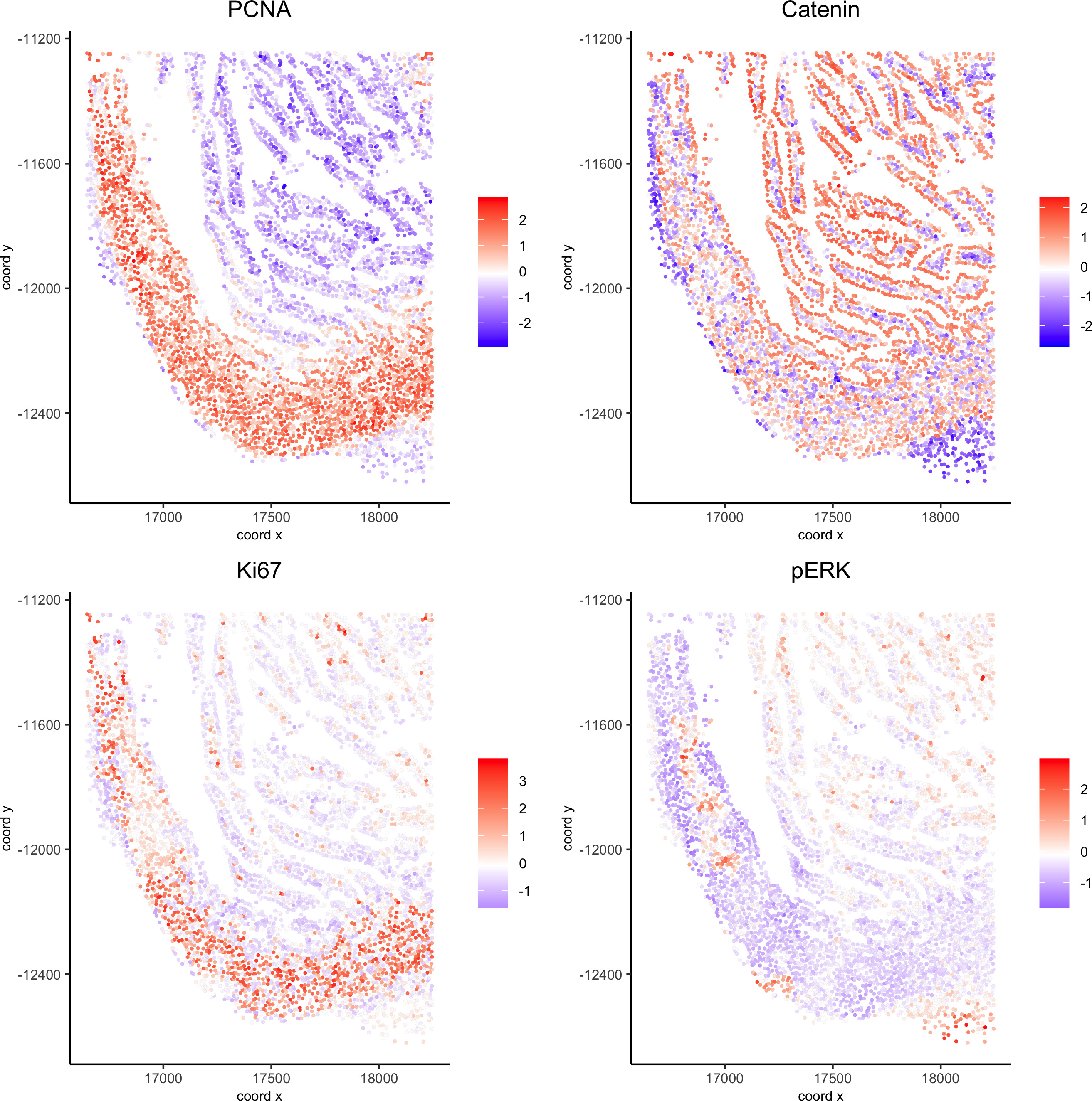
spatGenePlot(my_intest_giotto, expression_values = 'scaled', point_border_stroke = 0.01,genes = c('PCNA','Catenin', 'Ki67',  'pERK'), point_size = 1,save_param = list(save_name = 'xx_g_spatGeneplot'))

plotUMAP(my_intest_giotto, cell_color = 'leiden', point_shape = 'no_border', point_size = 0.5, 
cell_color_code = leiden_colors, show_center_label = F,save_param = list(save_name = 'xx_h_umap'))

dimGenePlot(my_intest_giotto, expression_values = 'scaled', point_border_stroke = 0.01,genes = c('PCNA','Catenin', 'Ki67',  'pERK'), point_size = 1,save_param = list(save_name = 'xx_i_dimGeneplot'))