10X Visium kidney dataset

0. Environment

library(Giotto)
# STOP!
# ====== 1. set working directory ======
# For Docker, set my_working_dir to /data
my_working_dir = '/data'
# For native install users, set my_working_dir to a directory accessible by user
#my_working_dir = "/home/qzhu/Downloads"
# ====== 2. set giotto python path ======
# For Docker, set python_path to /usr/bin/python3
python_path = "/usr/bin/python3"
# For native install users, python path may be different, and may depend on whether conda or virtual environment. One can check by "reticulate::py_discover_config()" to see which python is picked up automatically. Then set python_path to what is returned by py_discover_config.
# python_path = "/usr/bin/python3"

1. Dataset preparation steps

1.1. Dataset explanation

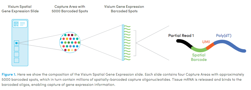
10X genomics recently launched a new platform to obtain spatial expression data using a Visium Spatial Gene Expression slide.

The Visium kidney data to run this tutorial can be found here

Visium technology:

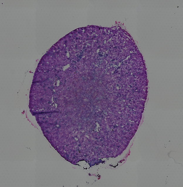
High resolution png from original tissue:

1.2. Dataset download

1.3. Giotto global instructions and preparations

## create instructions
instrs = createGiottoInstructions(save_dir = my_working_dir,save_plot = TRUE,show_plot = FALSE,python_path = python_path)
## provide path to visium folder
data_path = my_working_dir #containing raw_feature_bc_marix and spatial_folders

2. Create Giotto object & process data

## directly from visium folder
visium_kidney = createGiottoVisiumObject(visium_dir = data_path, expr_data = 'raw',png_name = 'tissue_lowres_image.png',gene_column_index = 2, instructions = instrs)
## update and align background image
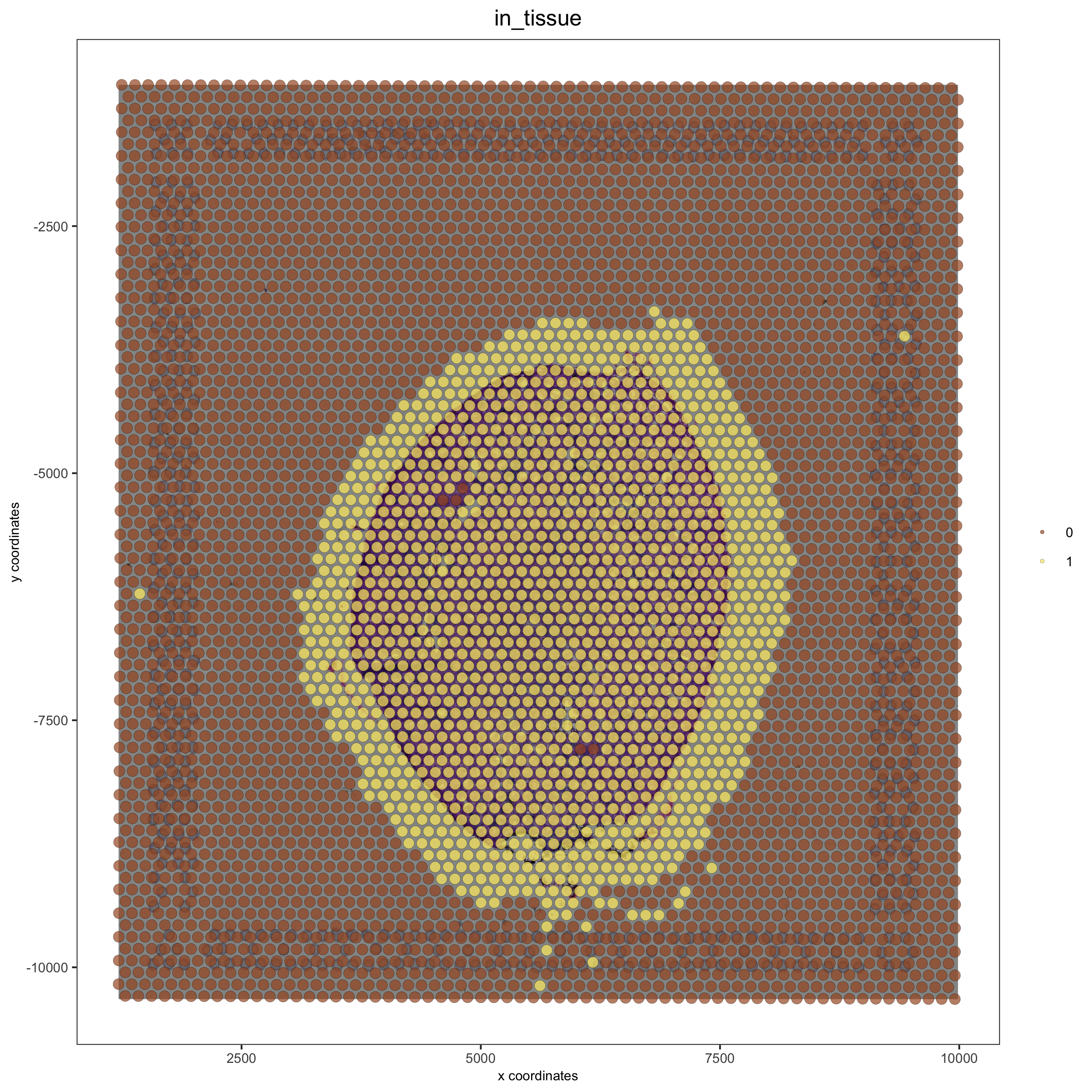
# problem: image is not perfectly aligned
spatPlot(gobject = visium_kidney, cell_color = 'in_tissue', show_image = T, point_alpha = 0.7,save_param = list(save_name = '2_a_spatplot_image'))

# check name
showGiottoImageNames(visium_kidney) # "image" is the default name
# adjust parameters to align image (iterative approach)
visium_kidney = updateGiottoImage(visium_kidney, image_name = 'image',xmax_adj = 1300, xmin_adj = 1200,ymax_adj = 1100, ymin_adj = 1000)
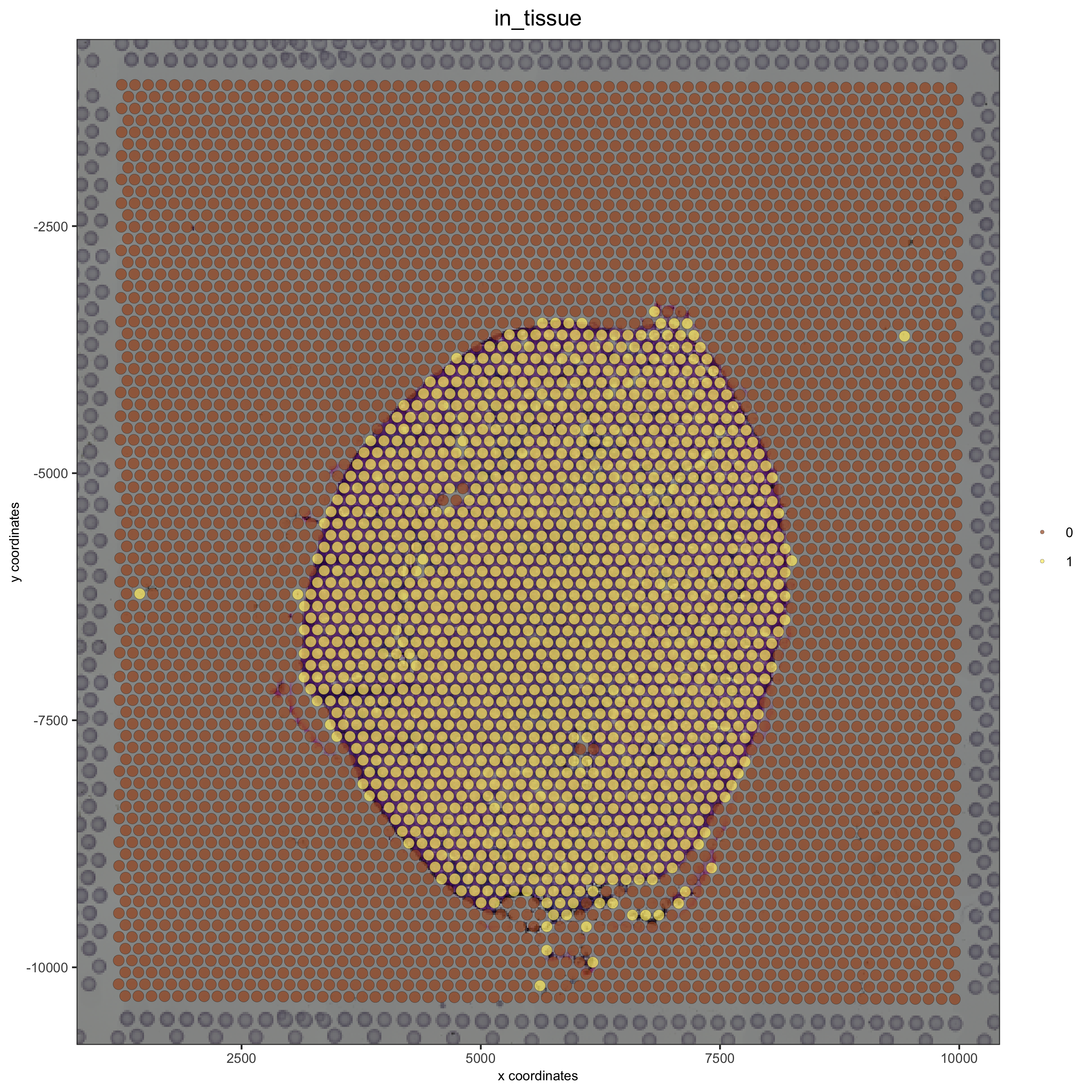
# now it's aligned
spatPlot(gobject = visium_kidney, cell_color = 'in_tissue', show_image = T, point_alpha = 0.7,save_param = list(save_name = '2_b_spatplot_image_adjusted'))

## check metadata
pDataDT(visium_kidney)
## compare in tissue with provided jpg
spatPlot(gobject = visium_kidney, cell_color = 'in_tissue', point_size = 2,cell_color_code = c('0' = 'lightgrey', '1' = 'blue'),save_param = list(save_name = '2_c_in_tissue'))

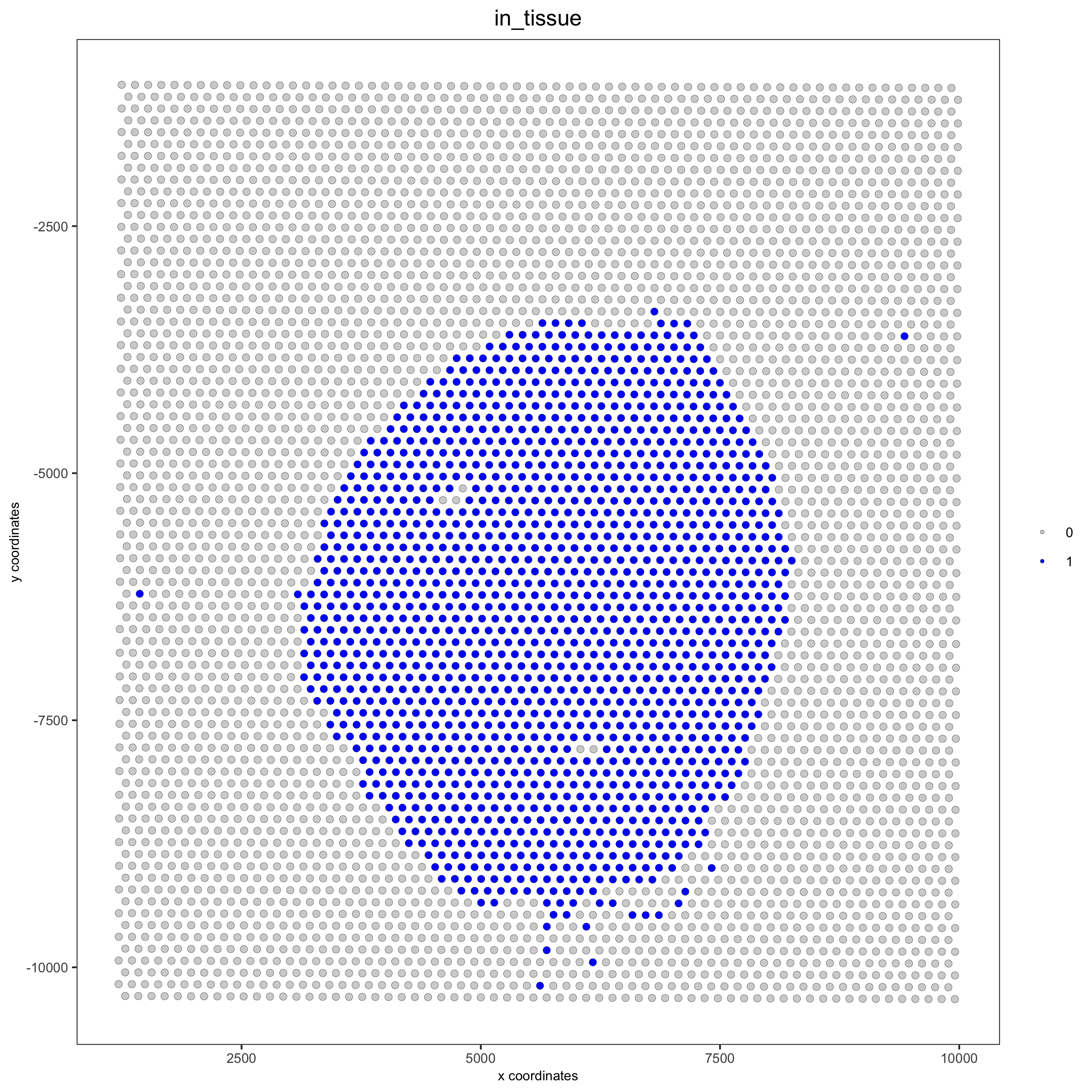
## subset on spots that were covered by tissue
metadata = pDataDT(visium_kidney)
in_tissue_barcodes = metadata[in_tissue == 1]$cell_ID
visium_kidney = subsetGiotto(visium_kidney, cell_ids = in_tissue_barcodes)
## filter
visium_kidney <- filterGiotto(gobject = visium_kidney,expression_threshold = 1,gene_det_in_min_cells = 50,min_det_genes_per_cell = 1000,expression_values = c('raw'),verbose = T)
## normalize
visium_kidney <- normalizeGiotto(gobject = visium_kidney, scalefactor = 6000, verbose = T)
## add gene & cell statistics
visium_kidney <- addStatistics(gobject = visium_kidney)
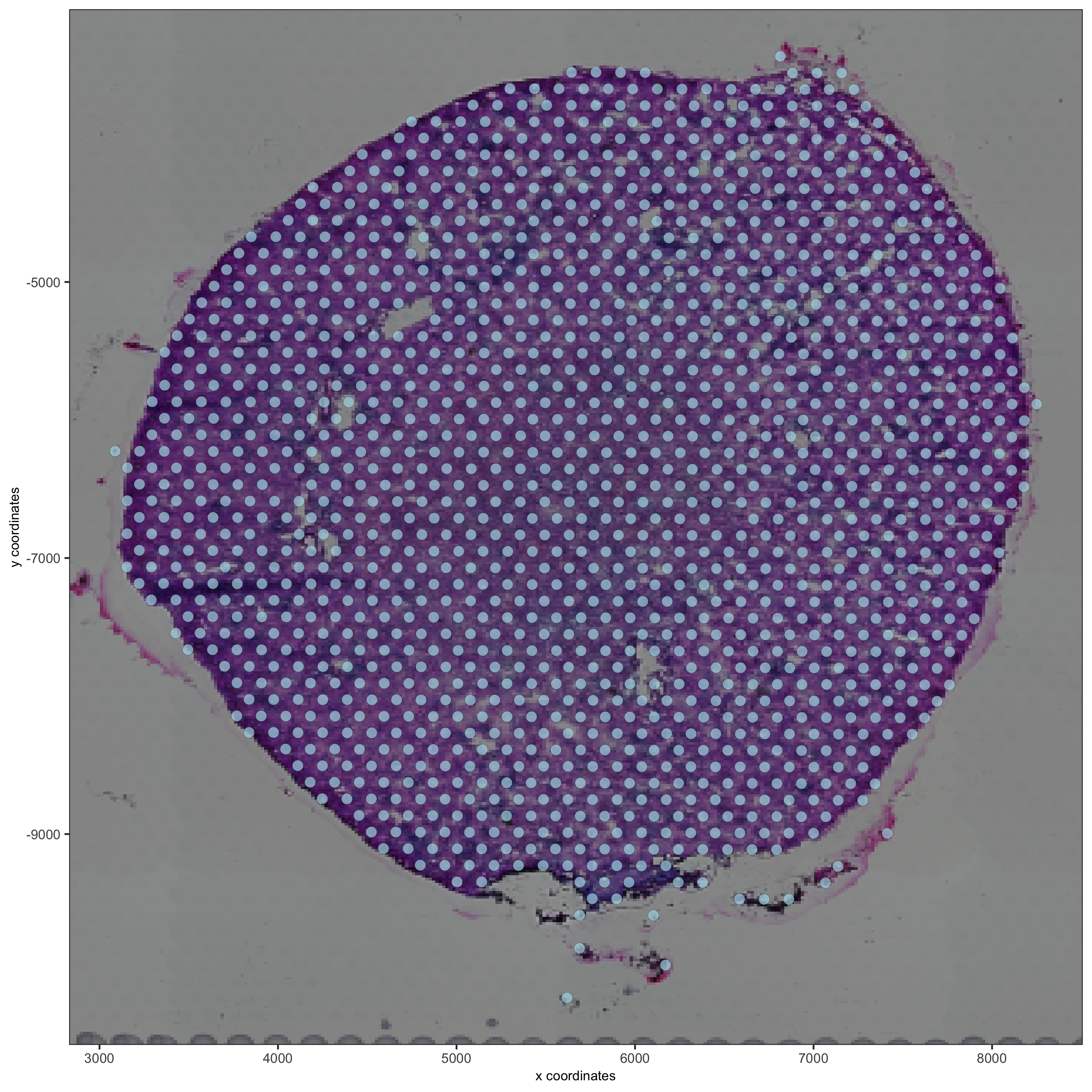
## visualize
spatPlot2D(gobject = visium_kidney, show_image = T, point_alpha = 0.7,save_param = list(save_name = '2_d_spatial_locations'))

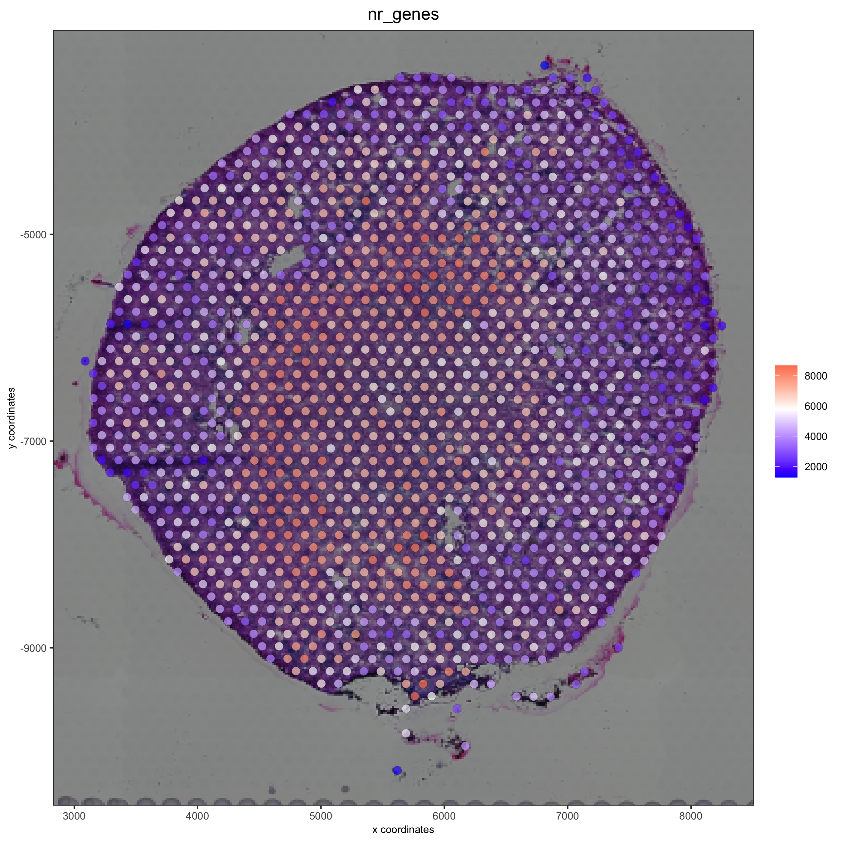
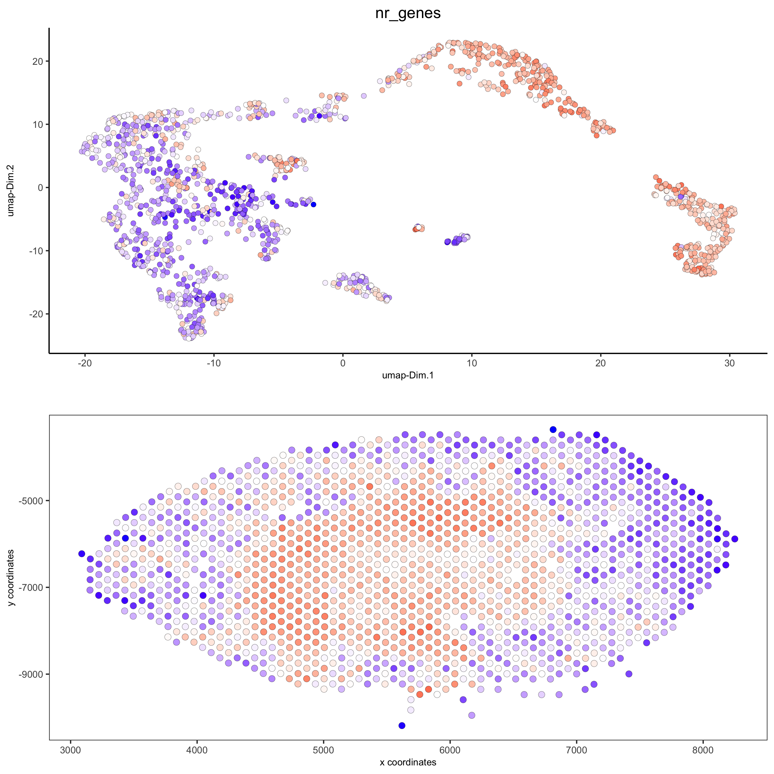
spatPlot2D(gobject = visium_kidney, show_image = T, point_alpha = 0.7,cell_color = 'nr_genes', color_as_factor = F,save_param = list(save_name = '2_e_nr_genes'))

3. Dimension reduction

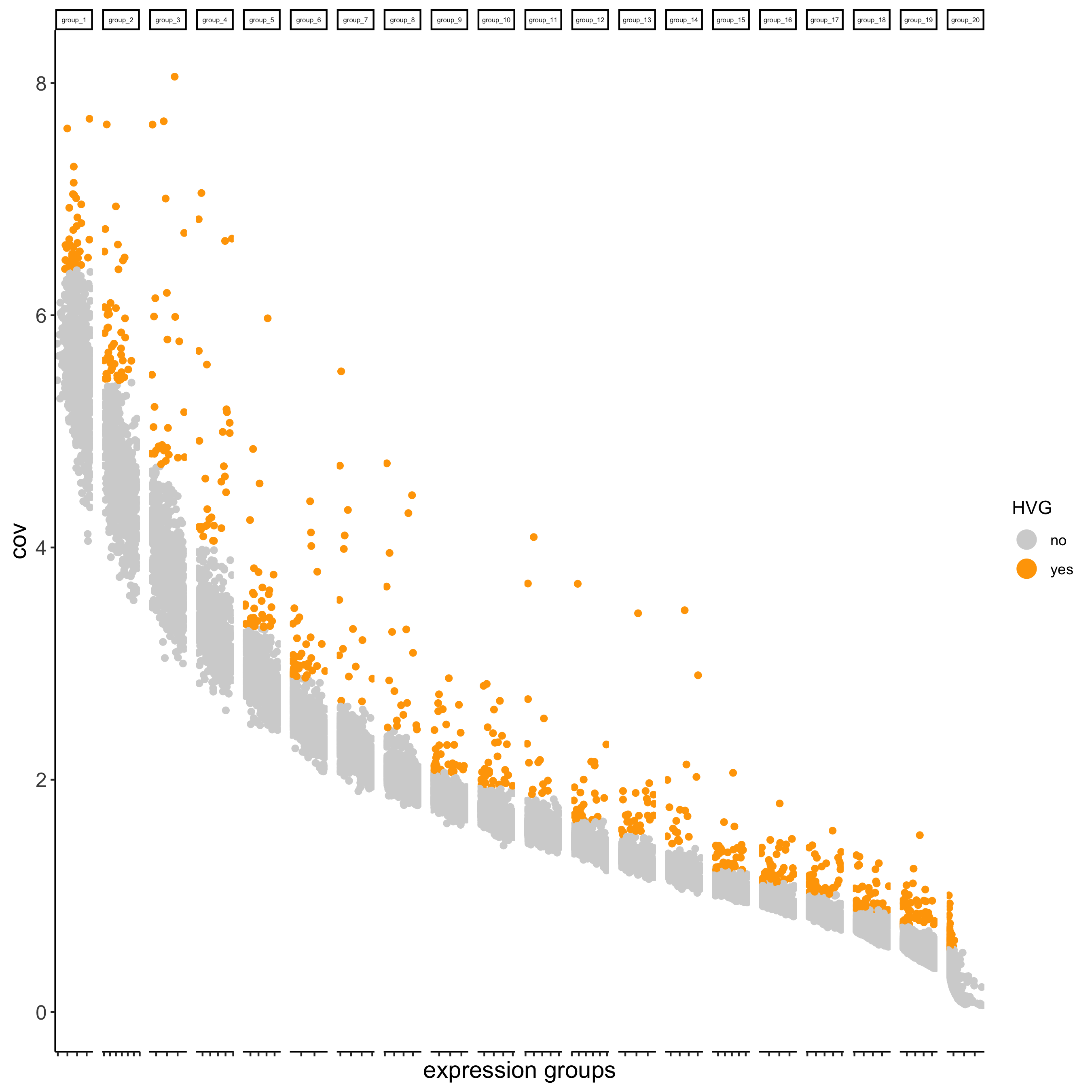
## highly variable genes (HVG)
visium_kidney <- calculateHVG(gobject = visium_kidney,save_param = list(save_name = '3_a_HVGplot'))

## run PCA on expression values (default)
visium_kidney <- runPCA(gobject = visium_kidney, center = TRUE, scale_unit = TRUE)
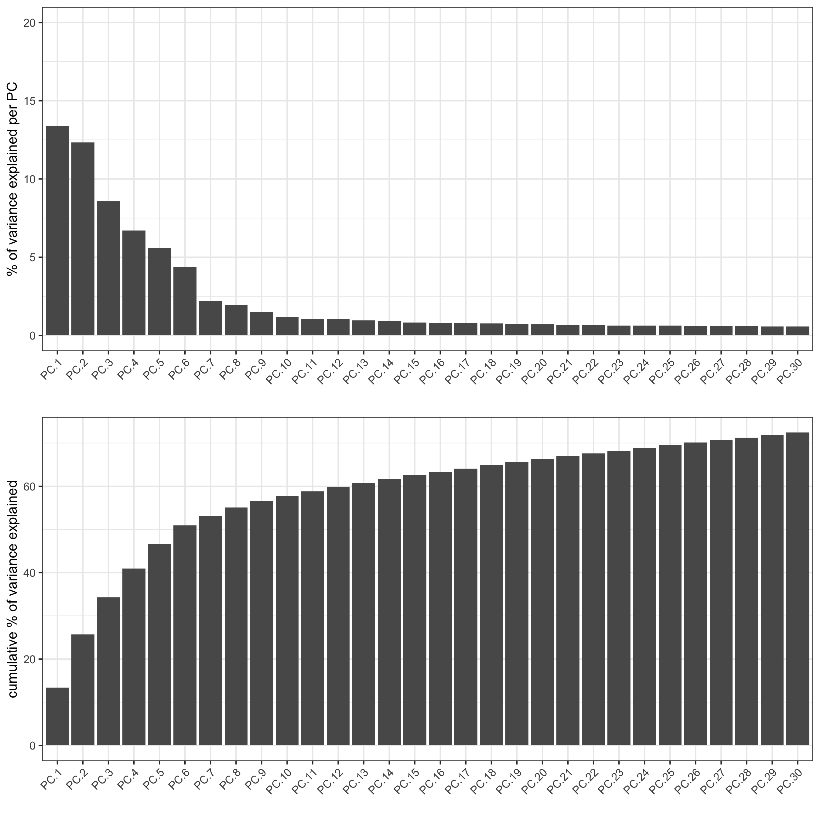
screePlot(visium_kidney, ncp = 30, save_param = list(save_name = '3_b_screeplot'))

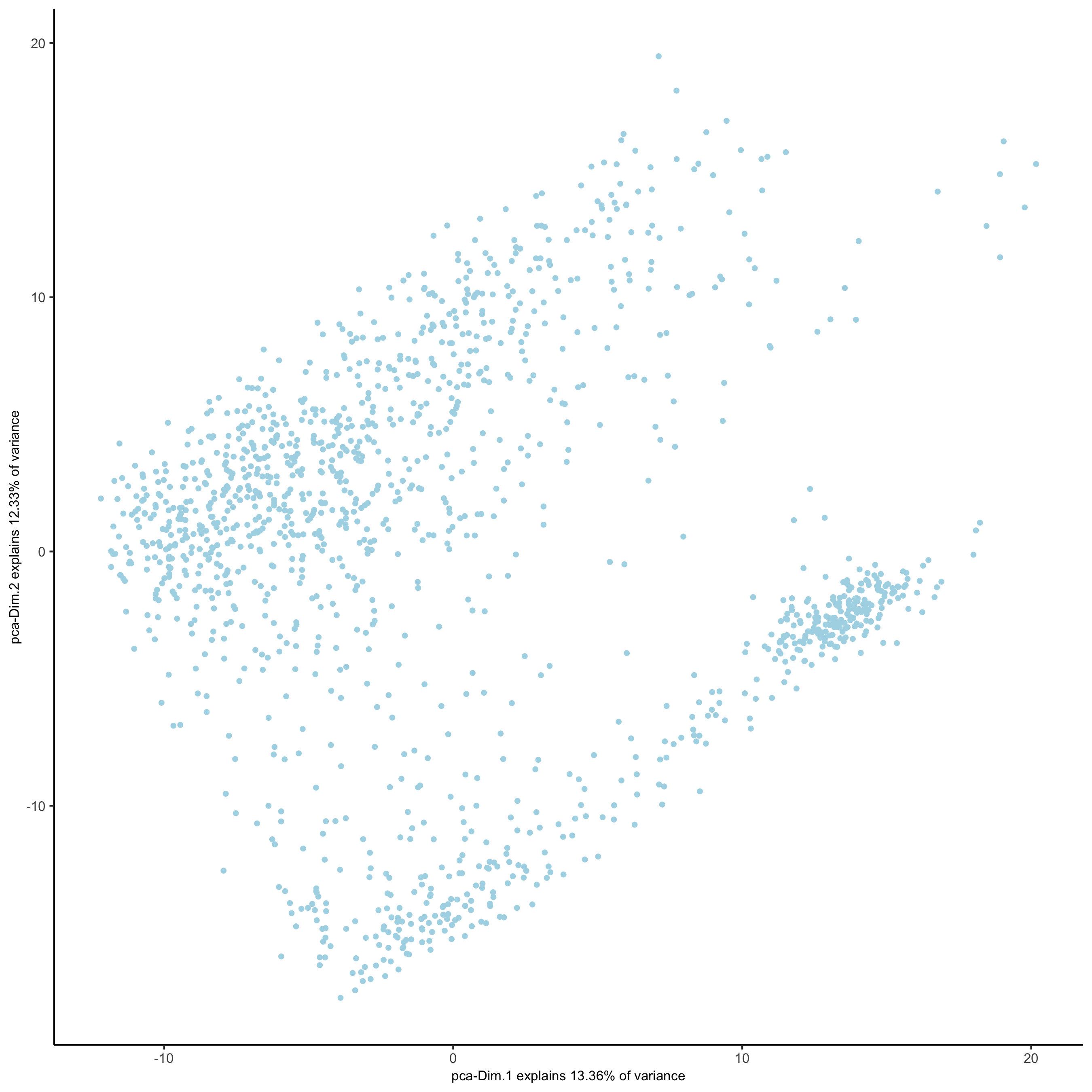
plotPCA(gobject = visium_kidney,save_param = list(save_name = '3_c_PCA_reduction'))

## run UMAP and tSNE on PCA space (default)
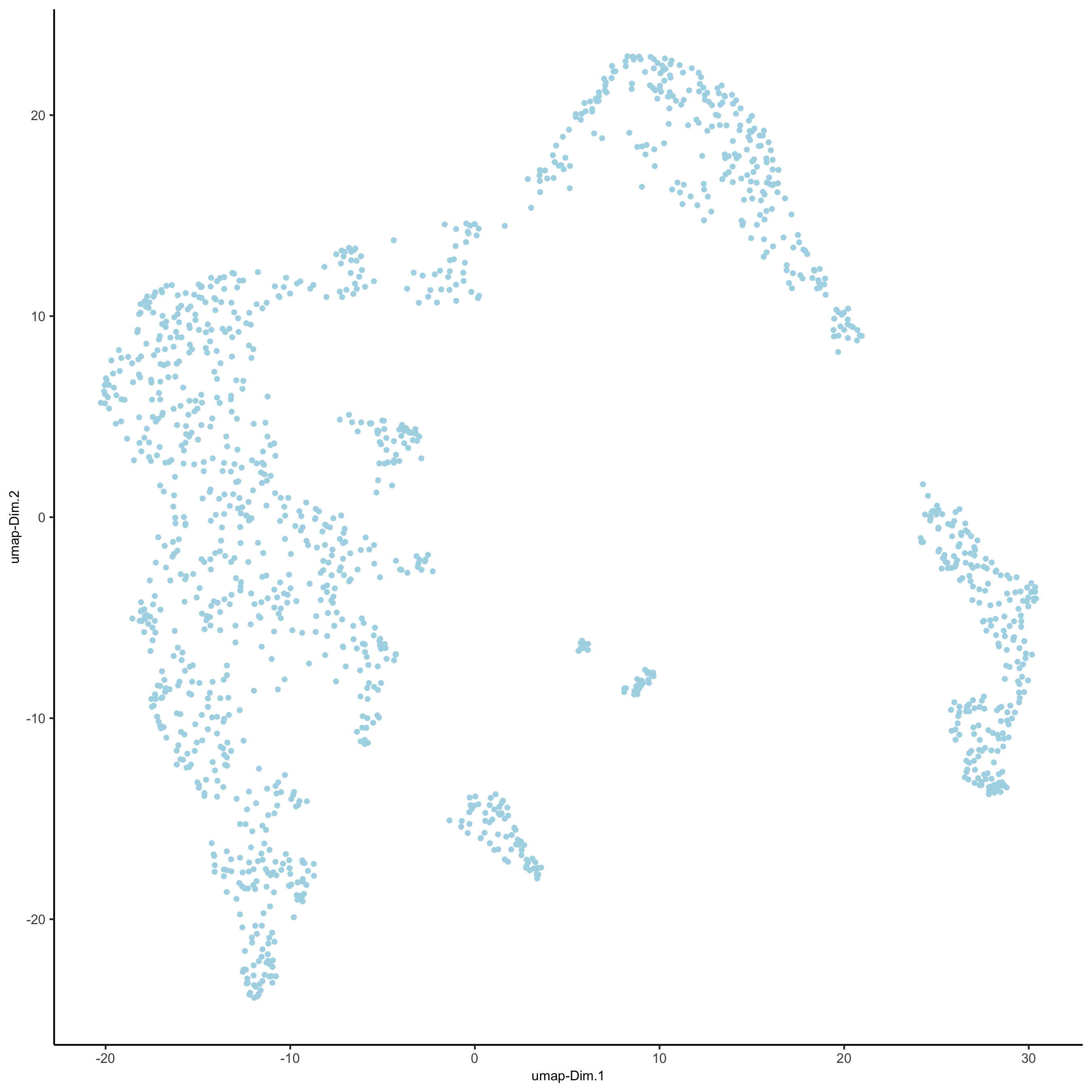
visium_kidney <- runUMAP(visium_kidney, dimensions_to_use = 1:10)
plotUMAP(gobject = visium_kidney,save_param = list(save_name = '3_d_UMAP_reduction'))

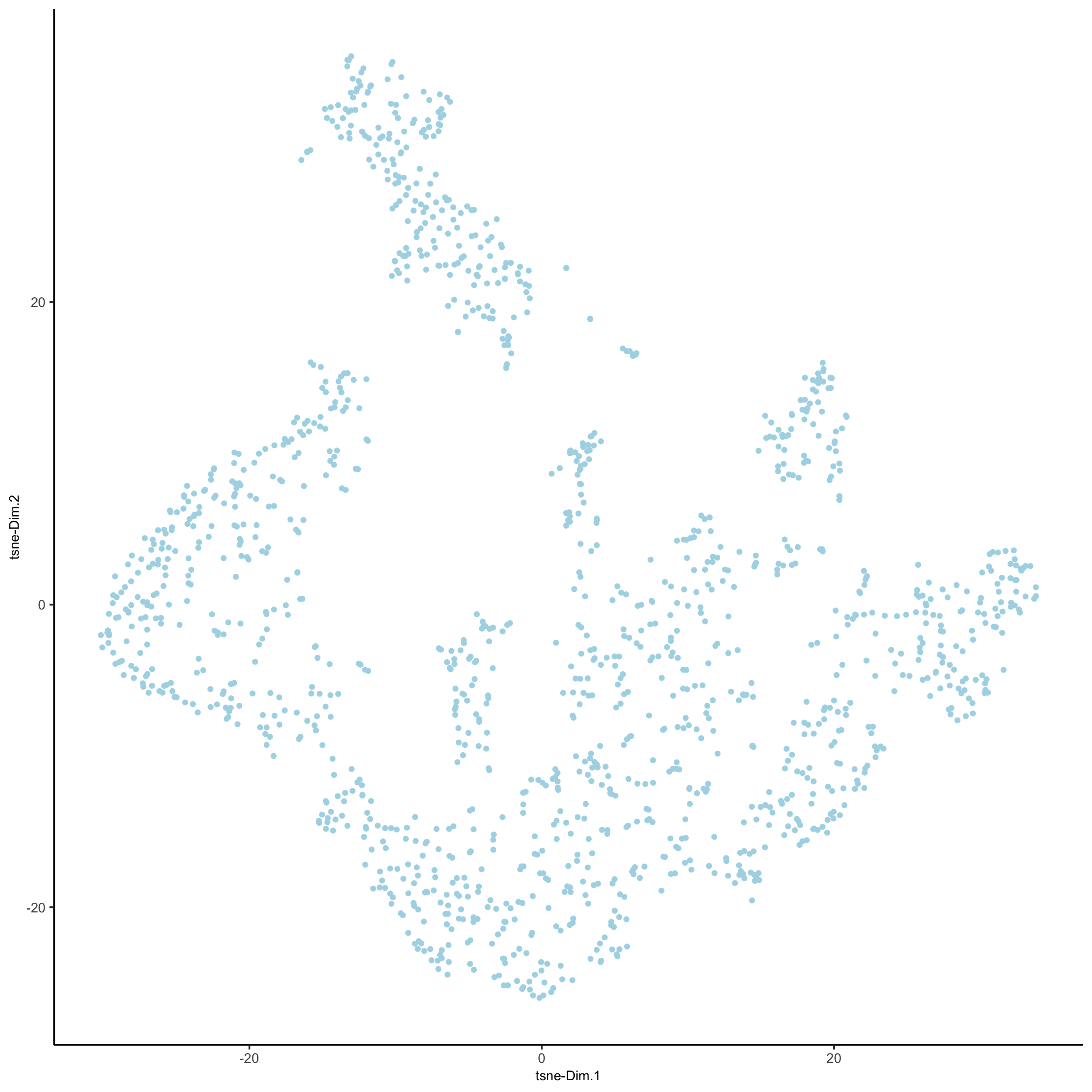
visium_kidney <- runtSNE(visium_kidney, dimensions_to_use = 1:10)
plotTSNE(gobject = visium_kidney,save_param = list(save_name = '3_e_tSNE_reduction'))

4. Cluster

## sNN network (default)
visium_kidney <- createNearestNetwork(gobject = visium_kidney, dimensions_to_use = 1:10, k = 15)
## Leiden clustering
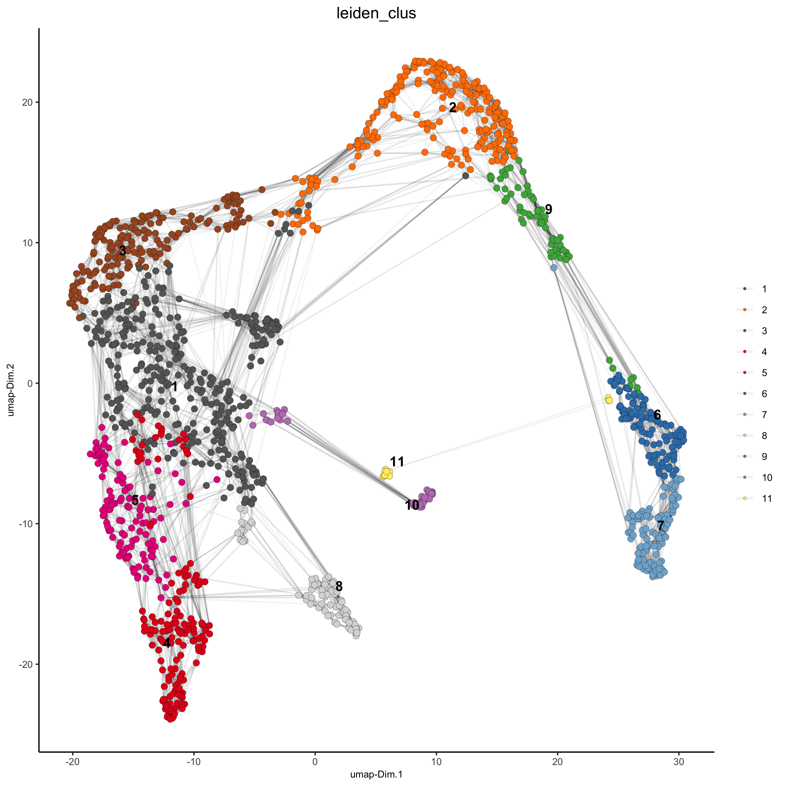
visium_kidney <- doLeidenCluster(gobject = visium_kidney, resolution = 0.4, n_iterations = 1000)
plotUMAP(gobject = visium_kidney,cell_color = 'leiden_clus', show_NN_network = T, point_size = 2.5,save_param = list(save_name = '4_a_UMAP_leiden'))

5. Co-visualize

# expression and spatial
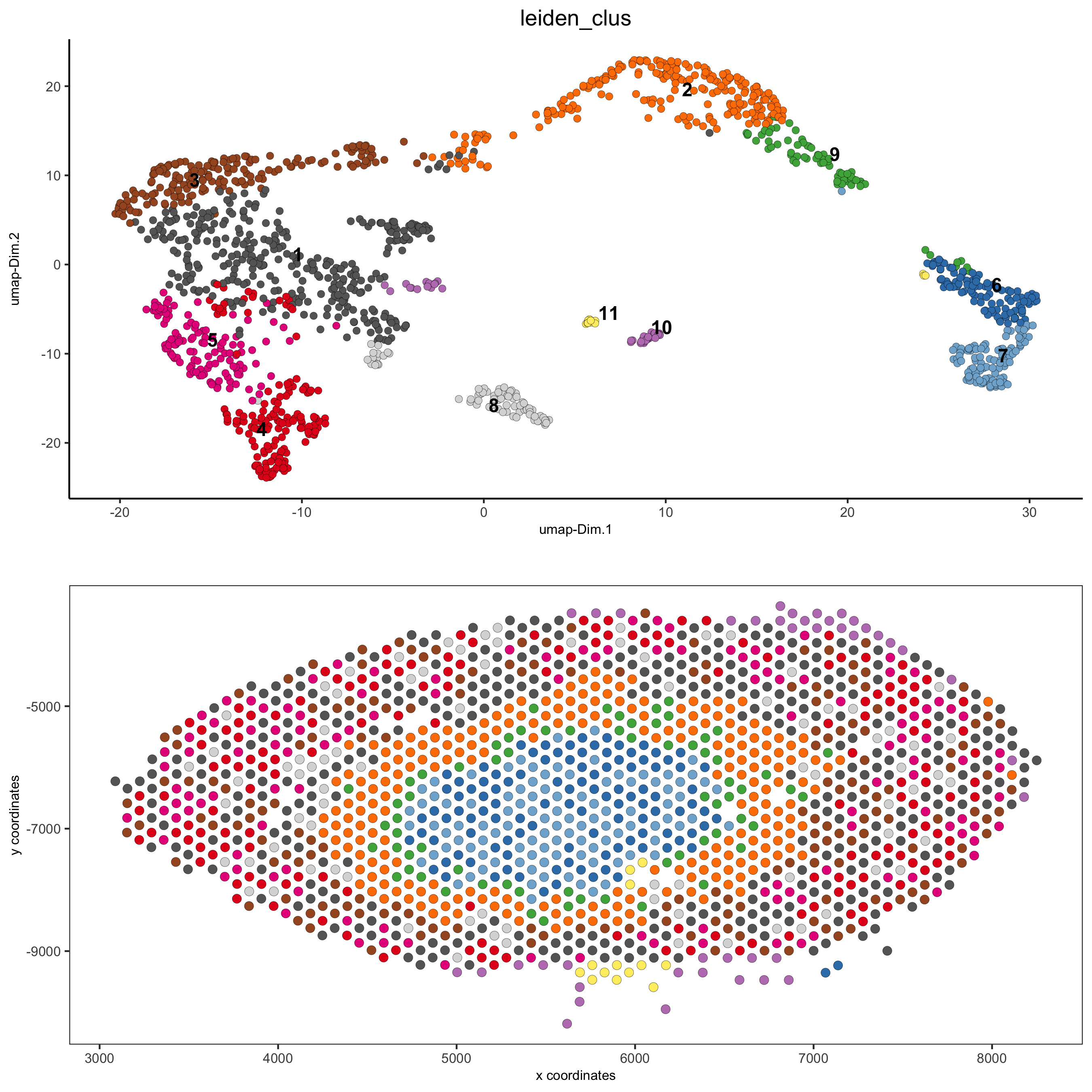
spatDimPlot(gobject = visium_kidney, cell_color = 'leiden_clus',dim_point_size = 2, spat_point_size = 2.5,save_param = list(save_name = '5_a_covis_leiden'))

spatDimPlot(gobject = visium_kidney, cell_color = 'nr_genes', color_as_factor = F,dim_point_size = 2, spat_point_size = 2.5,save_param = list(save_name = '5_b_nr_genes'))

6. Cell type marker gene detection

6.1. Gini

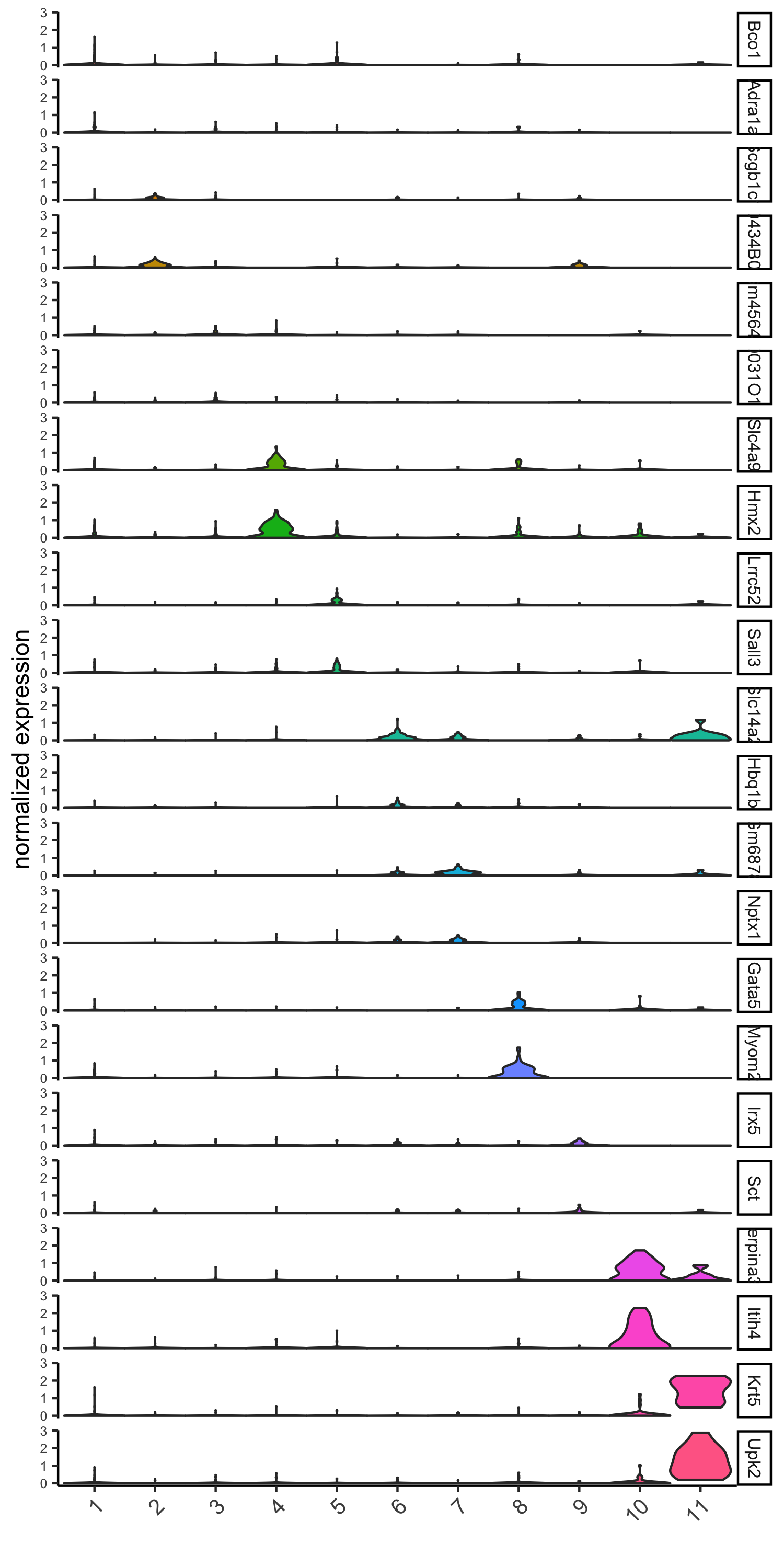
gini_markers_subclusters = findMarkers_one_vs_all(gobject = visium_kidney,method = 'gini',expression_values = 'normalized',cluster_column = 'leiden_clus',min_genes = 20,min_expr_gini_score = 0.5,min_det_gini_score = 0.5)
topgenes_gini = gini_markers_subclusters[, head(.SD, 2), by = 'cluster']$genes
# violinplot
violinPlot(visium_kidney, genes = unique(topgenes_gini), cluster_column = 'leiden_clus',strip_text = 8, strip_position = 'right',save_param = c(save_name = '6_a_violinplot_gini', base_width = 5, base_height = 10))

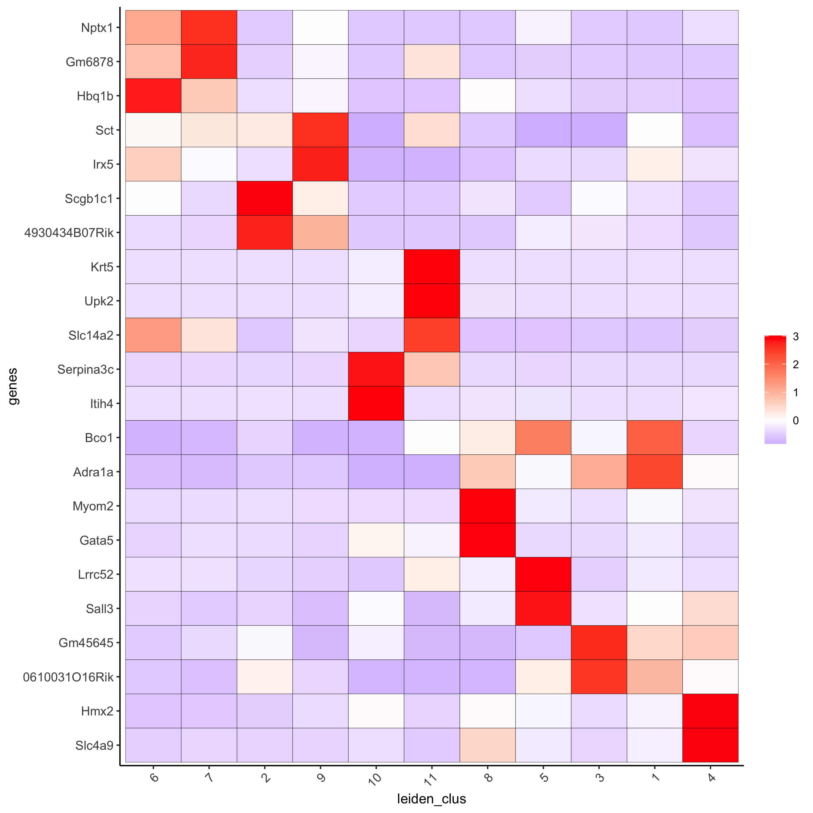
# cluster heatmap
plotMetaDataHeatmap(visium_kidney, selected_genes = topgenes_gini,metadata_cols = c('leiden_clus'), 
x_text_size = 10, y_text_size = 10,save_param = c(save_name = '6_b_metaheatmap_gini'))

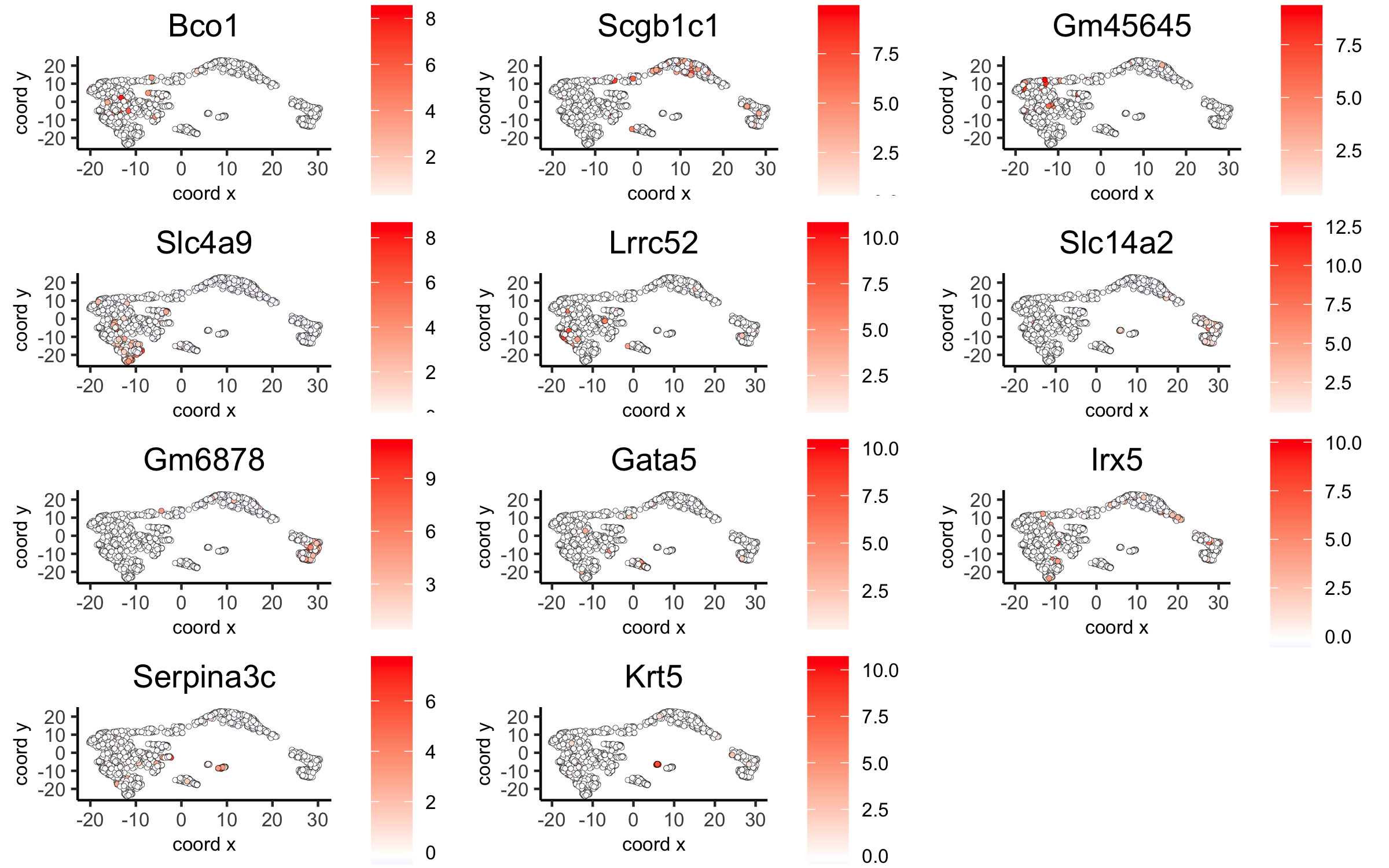
# umap plots
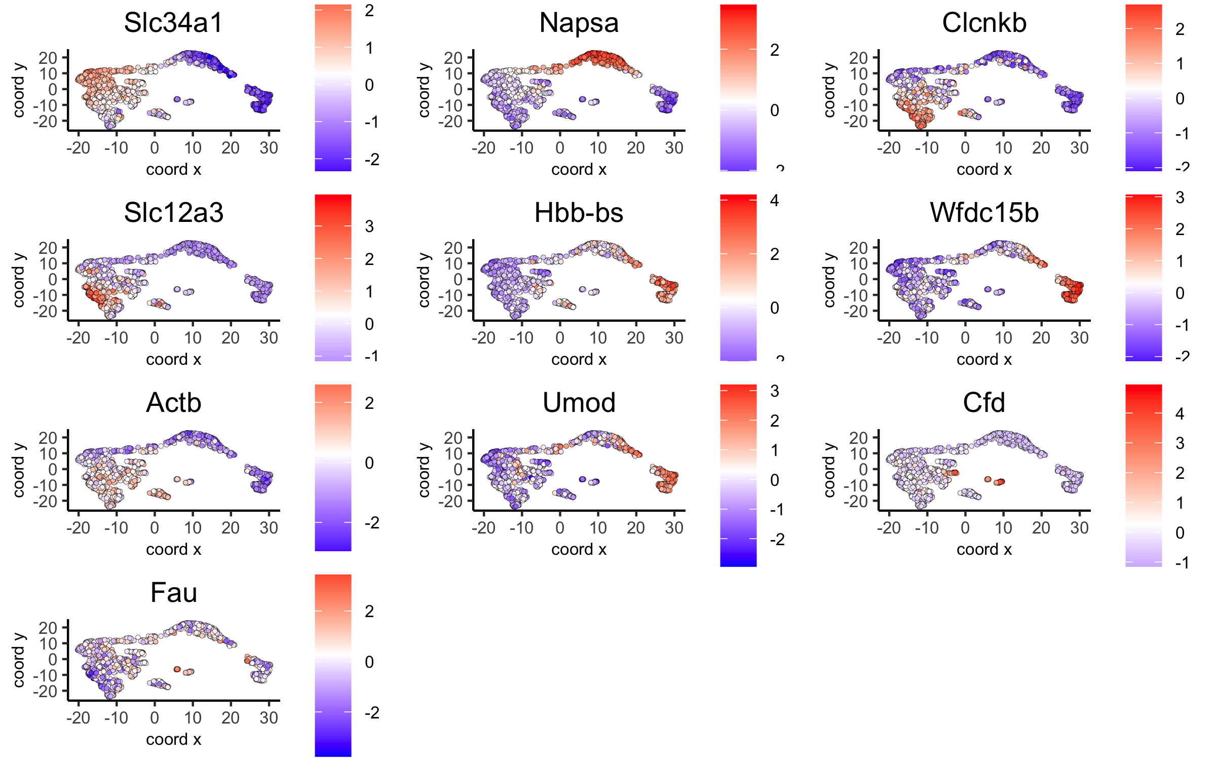
dimGenePlot2D(visium_kidney, expression_values = 'scaled',genes = gini_markers_subclusters[, head(.SD, 1), by = 'cluster']$genes,cow_n_col = 3, point_size = 1,save_param = c(save_name = '6_c_gini_umap', base_width = 8, base_height = 5))

6.2. Scran

scran_markers_subclusters = findMarkers_one_vs_all(gobject = visium_kidney,method = 'scran',expression_values = 'normalized',cluster_column = 'leiden_clus')
topgenes_scran = scran_markers_subclusters[, head(.SD, 2), by = 'cluster']$genes
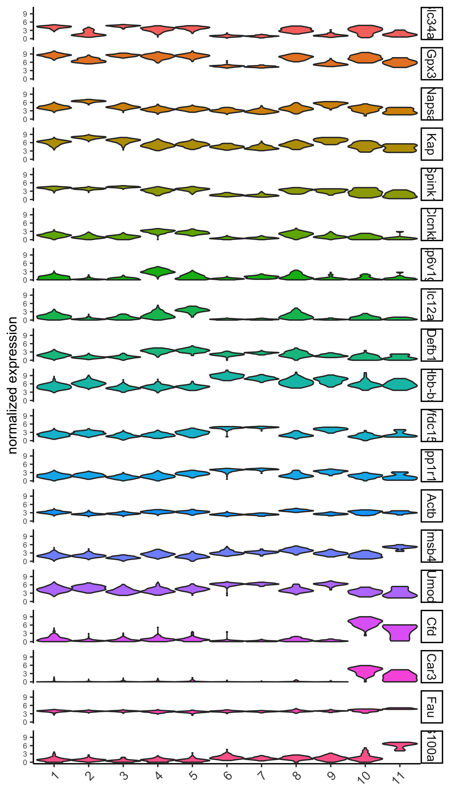
# violinplot
violinPlot(visium_kidney, genes = unique(topgenes_scran), cluster_column = 'leiden_clus',strip_text = 10, strip_position = 'right',save_param = c(save_name = '6_d_violinplot_scran', base_width = 5))

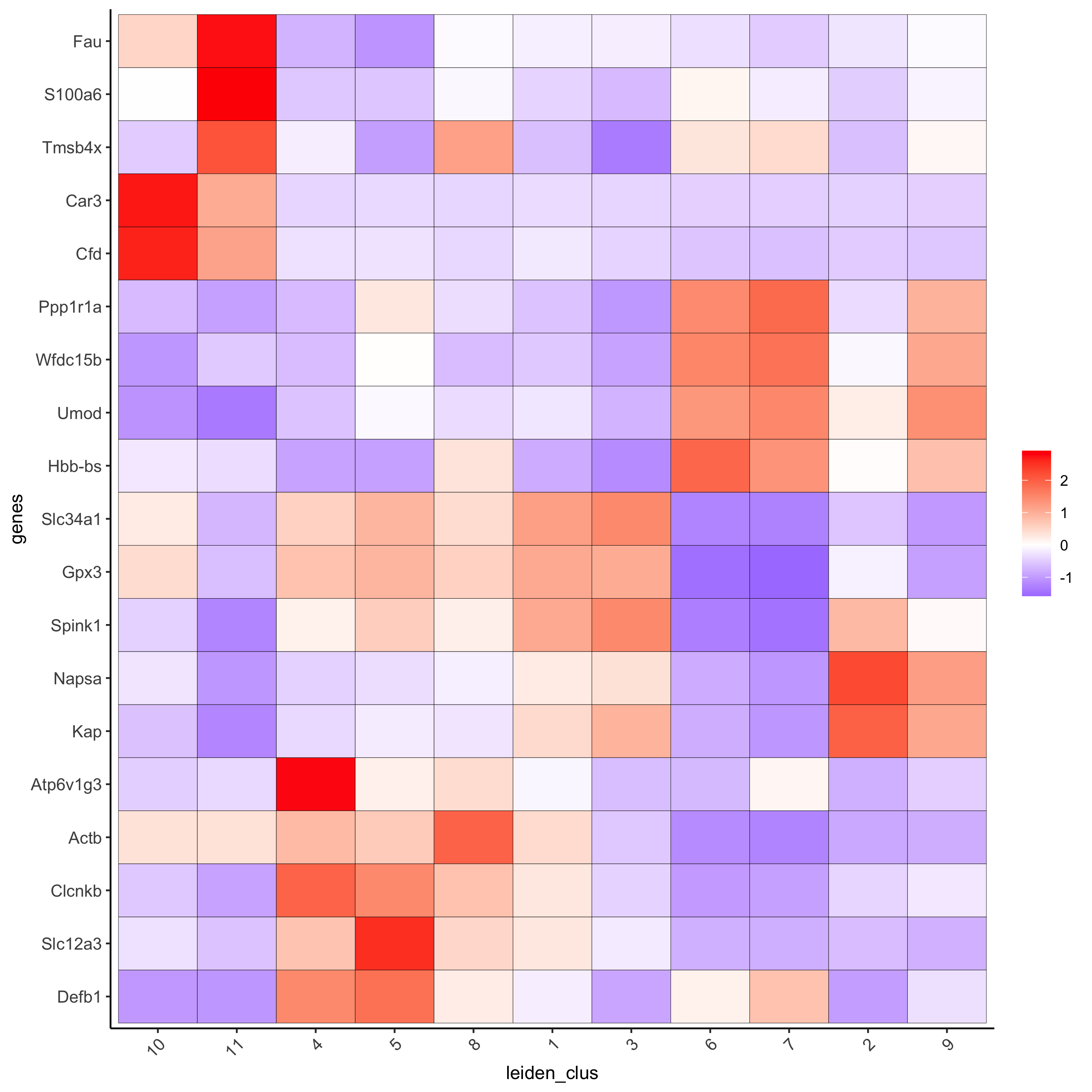
# cluster heatmap
plotMetaDataHeatmap(visium_kidney, selected_genes = topgenes_scran,metadata_cols = c('leiden_clus'),save_param = c(save_name = '6_e_metaheatmap_scran'))

# umap plots
dimGenePlot(visium_kidney, expression_values = 'scaled',genes = scran_markers_subclusters[, head(.SD, 1), by = 'cluster']$genes,cow_n_col = 3, point_size = 1,save_param = c(save_name = '6_f_scran_umap', base_width = 8, base_height = 5))

7. Cell-type annotation

Visium spatial transcriptomics does not provide single-cell resolution, making cell type annotation a harder problem. Giotto provides 3 ways to calculate enrichment of specific cell-type signature gene list:

• PAGE
  
• rank
  
• hypergeometric test

See the mouse Visium brain dataset for an example.

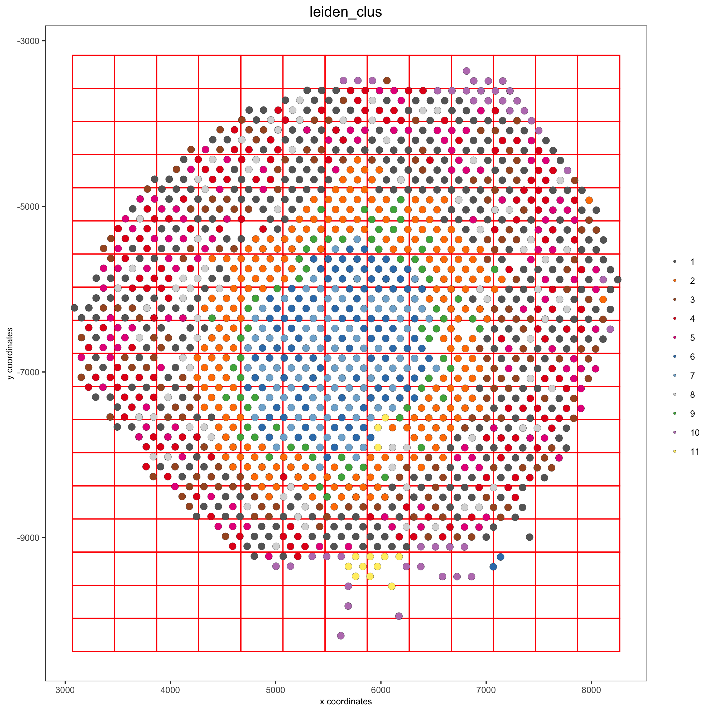
8. Spatial grid

visium_kidney <- createSpatialGrid(gobject = visium_kidney,sdimx_stepsize = 400,sdimy_stepsize = 400,minimum_padding = 0)
spatPlot(visium_kidney, cell_color = 'leiden_clus', show_grid = T,grid_color = 'red', spatial_grid_name = 'spatial_grid', 
save_param = c(save_name = '8_grid'))

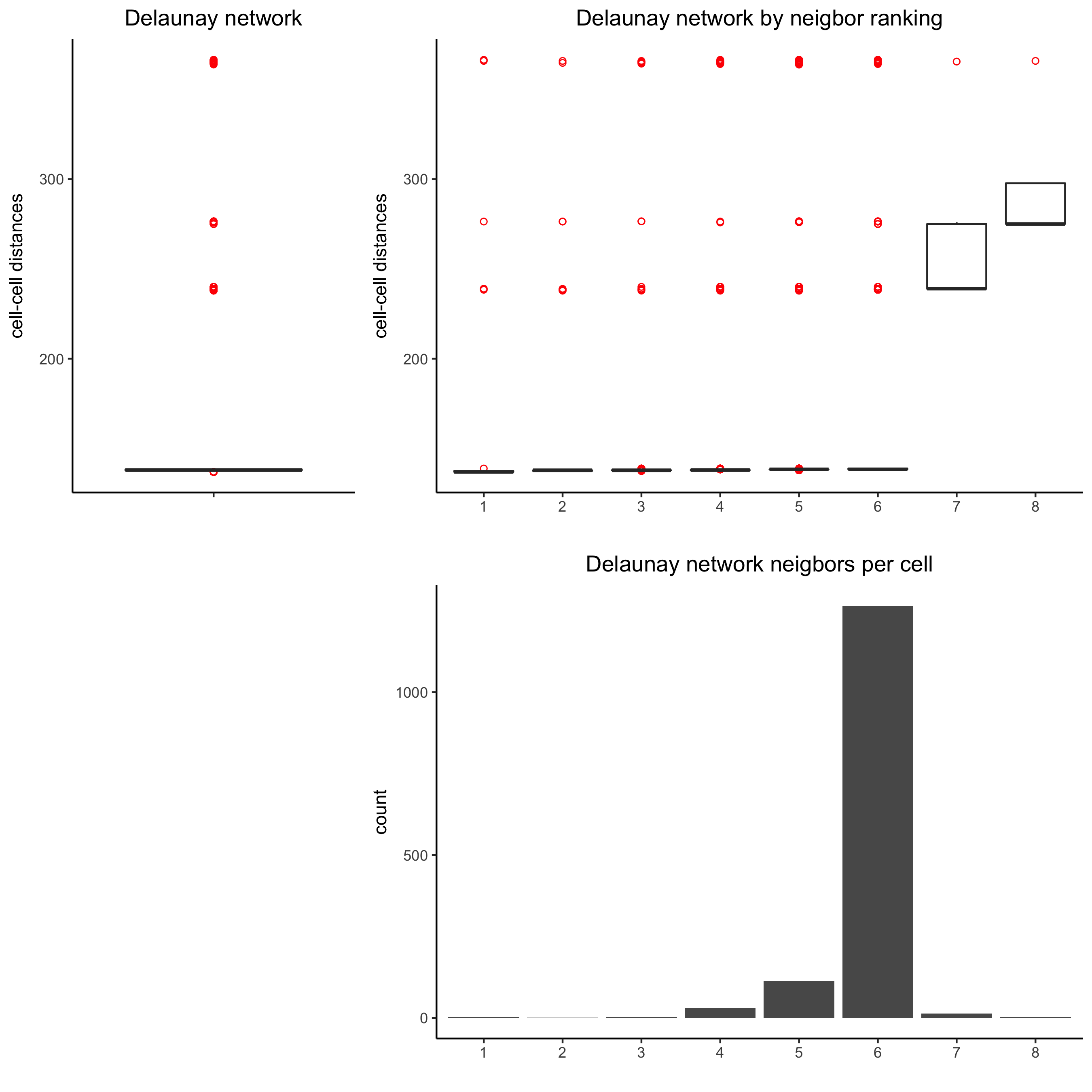
9. Spatial network

## delaunay network: stats + creation
plotStatDelaunayNetwork(gobject = visium_kidney, maximum_distance = 400, 
save_param = c(save_name = '9_a_delaunay_network'))

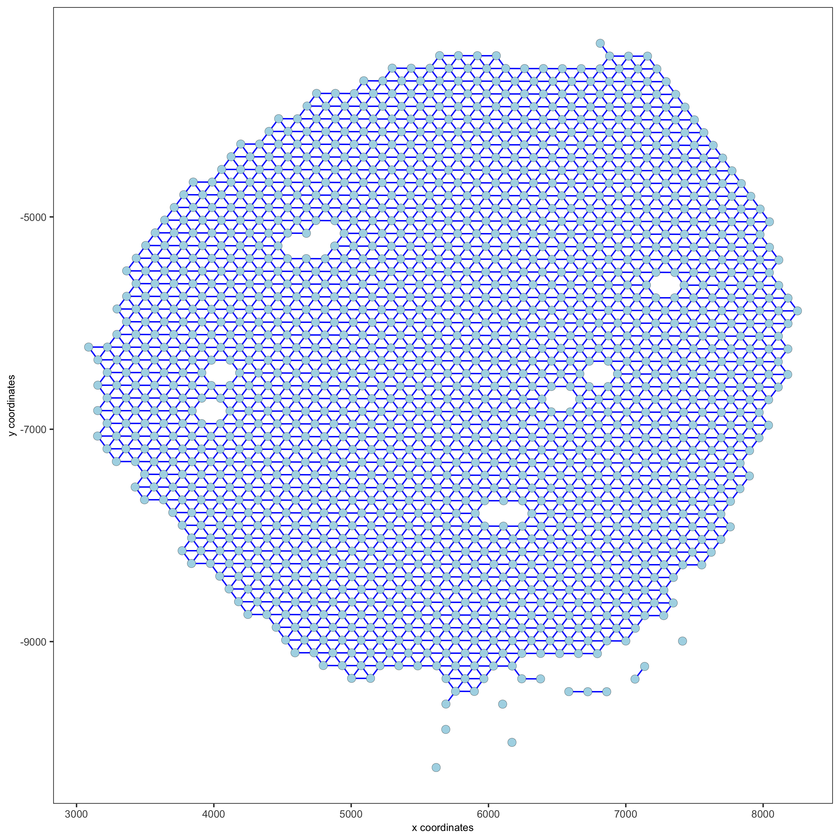
visium_kidney = createSpatialNetwork(gobject = visium_kidney, minimum_k = 0)
showNetworks(visium_kidney)
spatPlot(gobject = visium_kidney, show_network = T,network_color = 'blue', spatial_network_name = 'Delaunay_network',save_param = c(save_name = '9_b_delaunay_network'))

10. Spatial genes

10.1. Spatial genes

## kmeans binarization
kmtest = binSpect(visium_kidney)
spatGenePlot(visium_kidney, expression_values = 'scaled',genes = kmtest$genes[1:6], cow_n_col = 2, point_size = 1.5,save_param = c(save_name = '10_a_spatial_genes_km'))

## rank binarization
ranktest = binSpect(visium_kidney, bin_method = 'rank')
spatGenePlot(visium_kidney, expression_values = 'scaled',genes = ranktest$genes[1:6], cow_n_col = 2, point_size = 1.5,save_param = c(save_name = '10_b_spatial_genes_rank'))

10.2. Spatial co-expression patterns

## spatially correlated genes ##
ext_spatial_genes = kmtest[1:500]$genes
# 1. calculate gene spatial correlation and single-cell correlation 
# create spatial correlation object
spat_cor_netw_DT = detectSpatialCorGenes(visium_kidney, 
method = 'network', 
spatial_network_name = 'Delaunay_network',subset_genes = ext_spatial_genes)
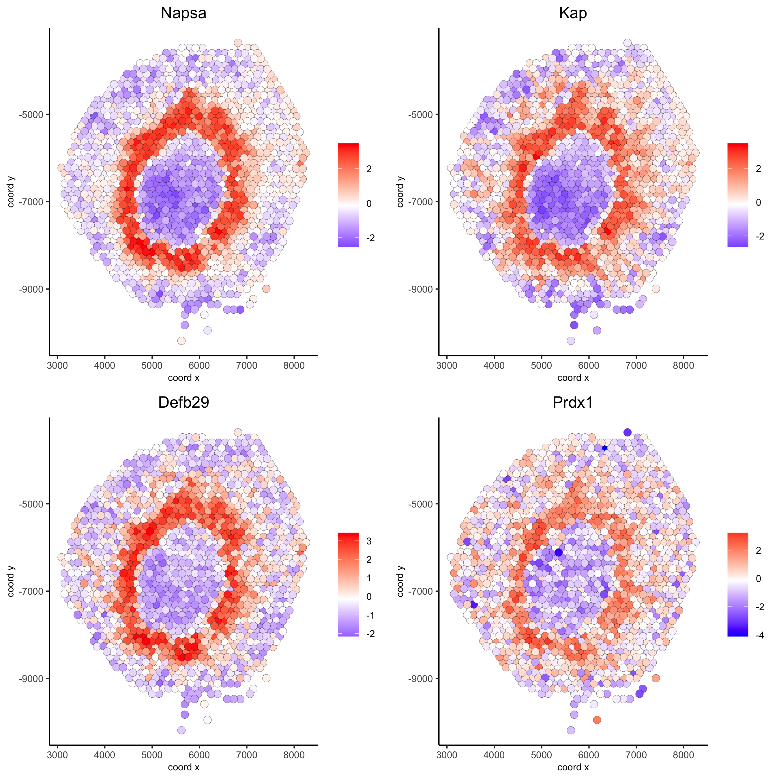
# 2. identify most similar spatially correlated genes for one gene
Napsa_top10_genes = showSpatialCorGenes(spat_cor_netw_DT, genes = 'Napsa', show_top_genes = 10)
spatGenePlot(visium_kidney, expression_values = 'scaled',genes = c('Napsa', 'Kap', 'Defb29', 'Prdx1'), point_size = 3,save_param = c(save_name = '10_d_Napsa_correlated_genes'))

# 3. cluster correlated genes & visualize
spat_cor_netw_DT = clusterSpatialCorGenes(spat_cor_netw_DT, name = 'spat_netw_clus', k = 8)
heatmSpatialCorGenes(visium_kidney, spatCorObject = spat_cor_netw_DT, use_clus_name = 'spat_netw_clus',save_param = c(save_name = '10_e_heatmap_correlated_genes', save_format = 'pdf',base_height = 6, base_width = 8, units = 'cm'), 
heatmap_legend_param = list(title = NULL))

# 4. rank spatial correlated clusters and show genes for selected clusters
netw_ranks = rankSpatialCorGroups(visium_kidney, spatCorObject = spat_cor_netw_DT, use_clus_name = 'spat_netw_clus',save_param = c(save_name = '10_f_rank_correlated_groups',base_height = 3, base_width = 5))

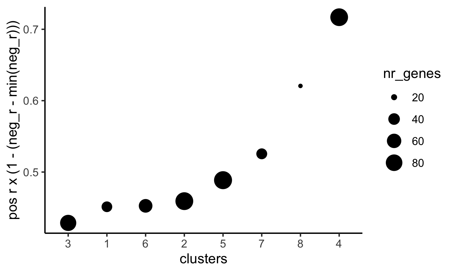
top_netw_spat_cluster = showSpatialCorGenes(spat_cor_netw_DT, use_clus_name = 'spat_netw_clus',selected_clusters = 6, show_top_genes = 1)
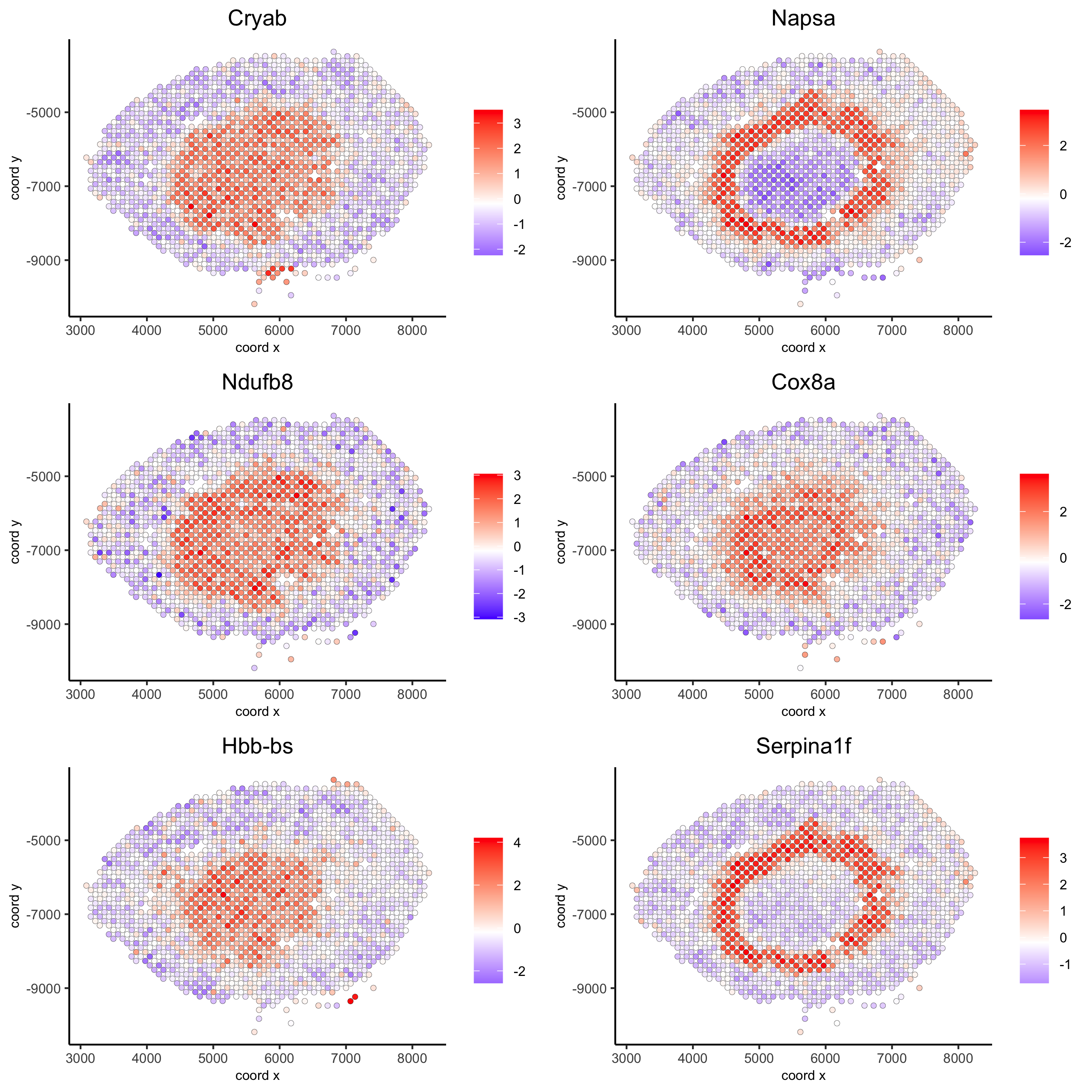
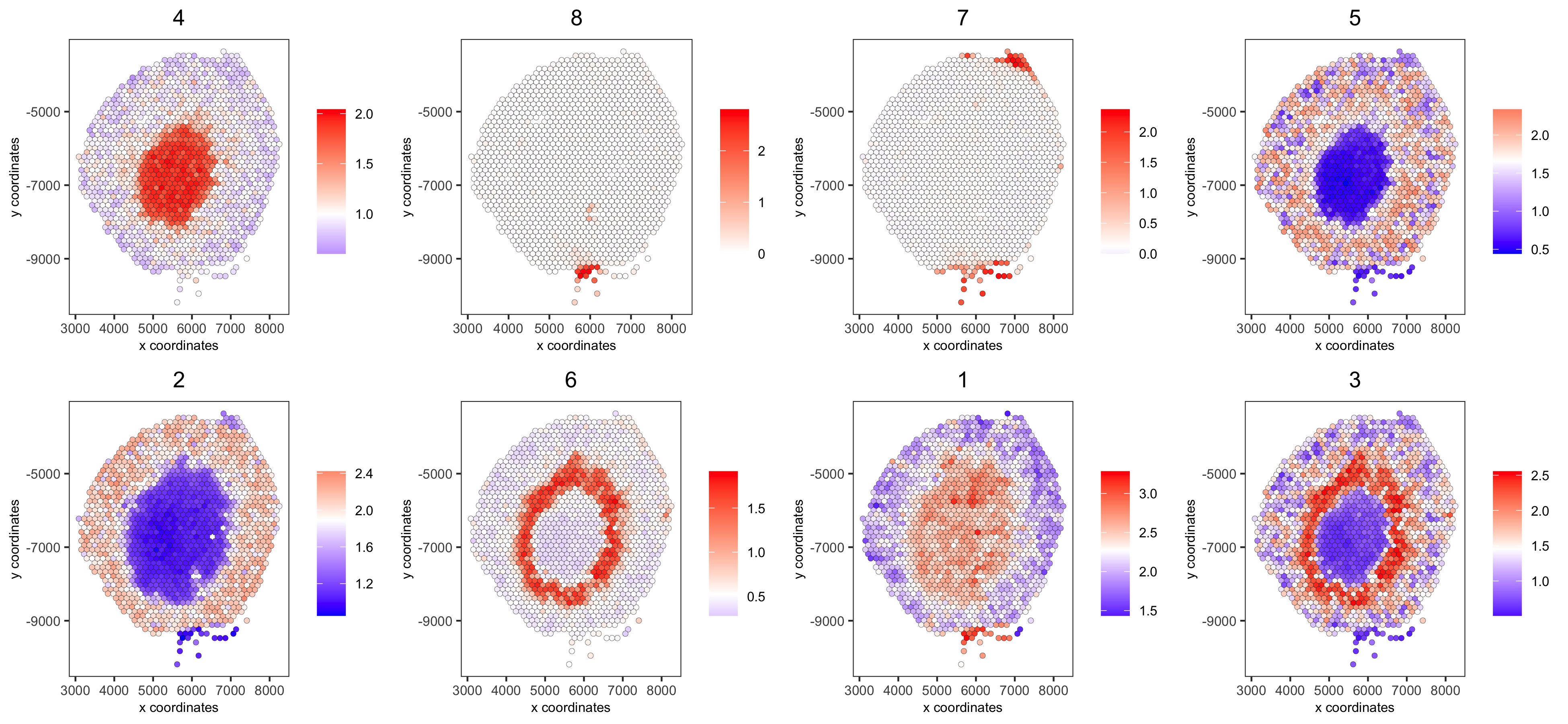
# 5. create metagene enrichment score for clusters
cluster_genes_DT = showSpatialCorGenes(spat_cor_netw_DT, use_clus_name = 'spat_netw_clus', show_top_genes = 1)
cluster_genes = cluster_genes_DT$clus; names(cluster_genes) = cluster_genes_DT$gene_ID
visium_kidney = createMetagenes(visium_kidney, gene_clusters = cluster_genes, name = 'cluster_metagene')
spatCellPlot(visium_kidney,spat_enr_names = 'cluster_metagene',cell_annotation_values = netw_ranks$clusters,point_size = 1.5, cow_n_col = 4, 
save_param = c(save_name = '10_g_spat_enrichment_score_plots',base_width = 13, base_height = 6))

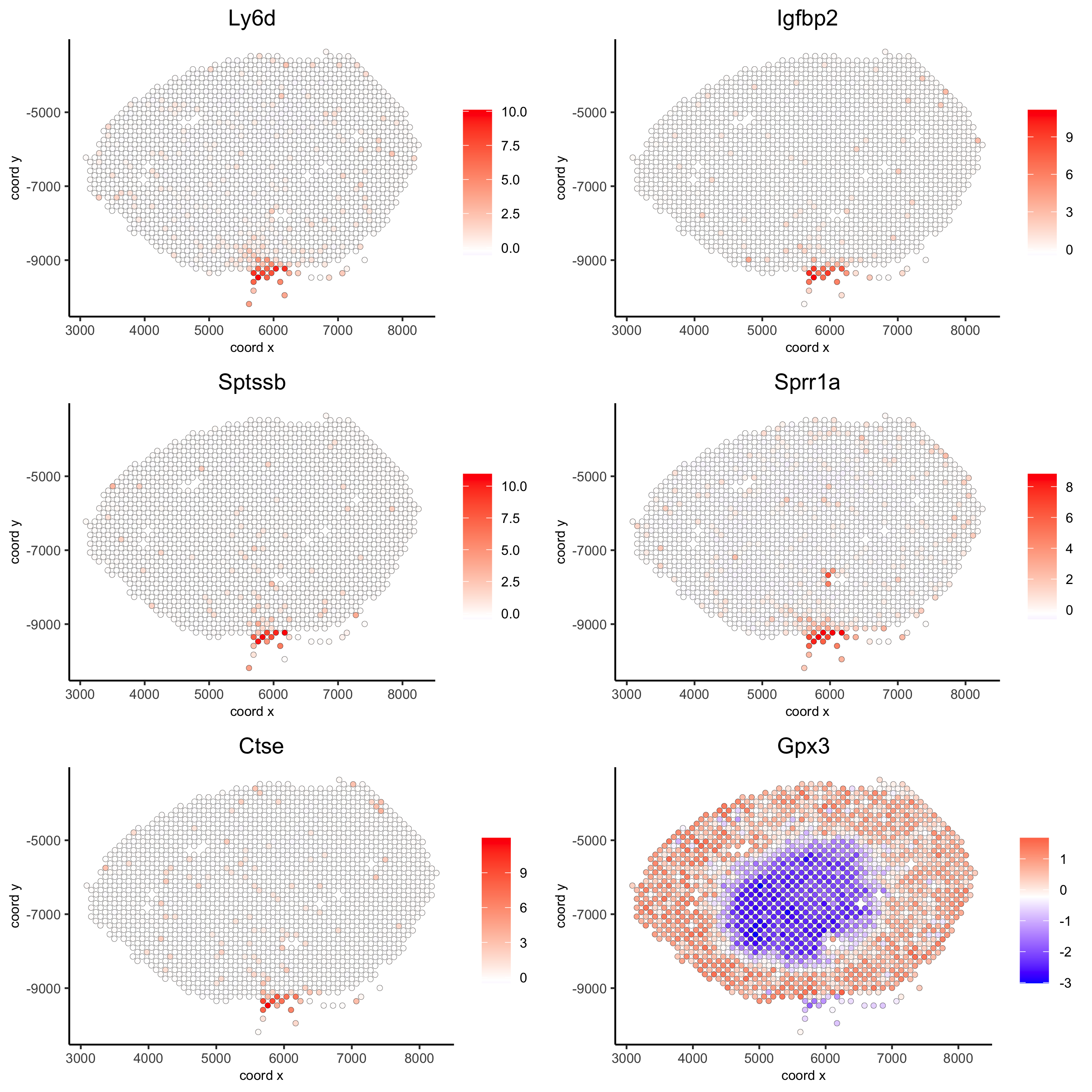
# example for gene per cluster
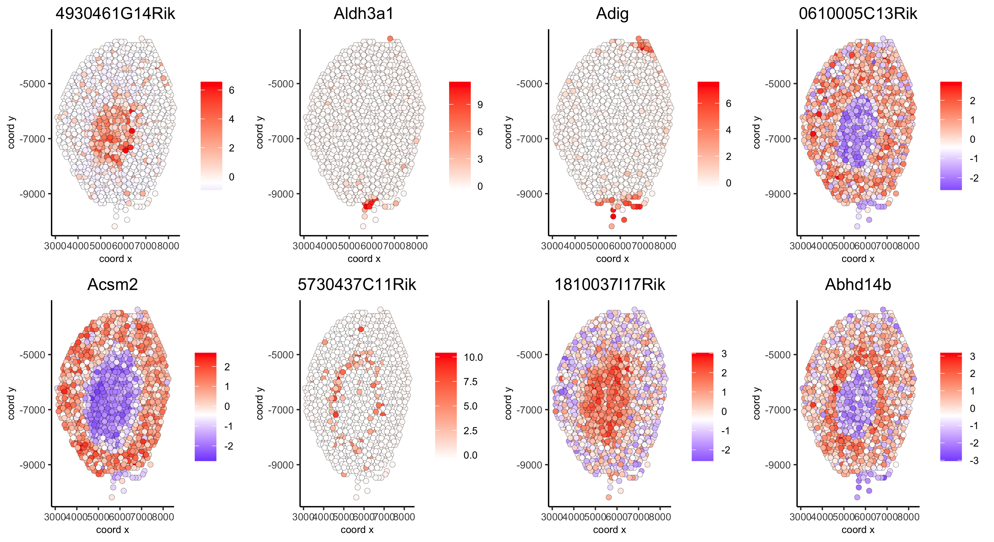
top_netw_spat_cluster = showSpatialCorGenes(spat_cor_netw_DT, use_clus_name = 'spat_netw_clus',selected_clusters = 1:8, show_top_genes = 1)
first_genes = top_netw_spat_cluster[, head(.SD, 1), by = clus]$gene_ID
cluster_names = top_netw_spat_cluster[, head(.SD, 1), by = clus]$clus
names(first_genes) = cluster_names
first_genes = first_genes[as.character(netw_ranks$clusters)]
spatGenePlot(visium_kidney, genes = first_genes, expression_values = 'scaled', cow_n_col = 4, midpoint = 0, point_size = 2,save_param = c(save_name = '10_h_spat_enrichment_score_plots_genes',base_width = 11, base_height = 6))

11. HMRF domains

# HMRF requires a fully connected network!
visium_kidney = createSpatialNetwork(gobject = visium_kidney, minimum_k = 2, name = 'Delaunay_full')
# spatial genes
my_spatial_genes <- kmtest[1:100]$genes
# do HMRF with different betas
hmrf_folder = fs::path(my_working_dir,'11_HMRF/')
if(!file.exists(hmrf_folder)) dir.create(hmrf_folder, recursive = T)
HMRF_spatial_genes = doHMRF(gobject = visium_kidney, expression_values = 'scaled', 
spatial_network_name = 'Delaunay_full',spatial_genes = my_spatial_genes,k = 5,betas = c(0, 1, 6), 
output_folder = fs::path(hmrf_folder, 'Spatial_genes/SG_topgenes_k5_scaled'))
## view results of HMRF
for(i in seq(0, 5, by = 1)) {
viewHMRFresults2D(gobject = visium_kidney,HMRFoutput = HMRF_spatial_genes,k = 5, betas_to_view = i,point_size = 2)
}

## alternative way to view HMRF results
#results = writeHMRFresults(gobject = ST_test,#                           HMRFoutput = HMRF_spatial_genes,#                           k = 5, betas_to_view = seq(0, 25, by = 5))
#ST_test = addCellMetadata(ST_test, new_metadata = results, by_column = T, column_cell_ID = 'cell_ID')
## add HMRF of interest to giotto object
visium_kidney = addHMRF(gobject = visium_kidney,HMRFoutput = HMRF_spatial_genes,k = 5, betas_to_add = c(0, 2),hmrf_name = 'HMRF')
## visualize
spatPlot(gobject = visium_kidney, cell_color = 'HMRF_k5_b.0', point_size = 5,save_param = c(save_name = '11_a_HMRF_k5_b.0'))

spatPlot(gobject = visium_kidney, cell_color = 'HMRF_k5_b.2', point_size = 5,save_param = c(save_name = '11_b_HMRF_k5_b.2'))

12. Export and create Giotto Viewer

# check which annotations are available
combineMetadata(visium_kidney)
# select annotations, reductions and expression values to view in Giotto Viewer
viewer_folder = fs::path(my_working_dir, 'mouse_visium_kidney_viewer')
exportGiottoViewer(gobject = visium_kidney,output_directory = viewer_folder,spat_enr_names = 'PAGE', 
factor_annotations = c('in_tissue','leiden_clus'),numeric_annotations = c('nr_genes','clus_25'),dim_reductions = c('tsne', 'umap'),dim_reduction_names = c('tsne', 'umap'),expression_values = 'scaled',expression_rounding = 2,overwrite_dir = T)

#================================================================ 
#Next steps. Please manually run the following in a SHELL terminal: 
#================================================================ 
cd  /data/mouse_visium_kidney_viewer 
giotto_setup_image --require-stitch=n --image=n --image-multi-channel=n --segmentation=n --multi-fov=n --output-json=step1.json 
smfish_step1_setup -c step1.json 
giotto_setup_viewer --num-panel=2 --input-preprocess-json=step1.json --panel-1=PanelPhysicalSimple --panel-2=PanelTsne --output-json=step2.json --input-annotation-list=annotation_list.txt 
smfish_read_config -c step2.json -o test.dec6.js -p test.dec6.html -q test.dec6.css 
giotto_copy_js_css --output . 
python3 -m http.server 
================================================================ 
#Finally, open your browser, navigate to http://localhost:8000/. Then click on the file test.dec6.html to see the viewer.