slideSeq Dataset - Part 1. Cell Type Enrichment

0. Environment

library(Giotto)
# STOP!
# ====== 1. set working directory ======
# For Docker, set my_working_dir to /data
my_working_dir = '/data'
# For native install users, set my_working_dir to a directory accessible by user
#my_working_dir = "/home/qzhu/Downloads"
# ====== 2. set giotto python path ======
# For Docker, set python_path to /usr/bin/python3
python_path = "/usr/bin/python3"
# For native install users, python path may be different, and may depend on whether conda or virtual environment. One can check by "reticulate::py_discover_config()" to see which python is picked up automatically. Then set python_path to what is returned by py_discover_config.
# python_path = "/usr/bin/python3"

1. Dataset preparation steps

1.1. Dataset explanations

This section will illustrate the cell type enrichment analysis. We will start with the scRNAseq dataset, perform clustering to find cell types, show how to generate cell type signature matrix to be used for cell type enrichment. Finally, we will apply on the slideSeq cerebellum dataset to deconvolve cell types in individual beads. In the analysis of scRNAseq, the input is the count matrix (single-cell). No cell type information is needed.

1.2. Single-cell RNAseq

To define cell types, we will need single-cell RNAseq dataset. Giotto can be used to analyze scRNAseq as well. The scRNAseq comes from http://mousebrain.org/ from the the Linnarsson Lab. We will use the cerebellum portion of the atlas in counts.

1.3. Dataset download

2. Processing and analyses of scRNAseq dataset

expr=read.table(fs::path(my_working_dir, "l1.cerebellum.txt"))
cell_names=data.table::fread(fs::path(my_working_dir, "l1.cerebellum.cellID.txt"), header=F)
gene_names=data.table::fread(fs::path(my_working_dir, "l1.cerebellum.genes.txt"), header=F)
gene_names[, dupl := duplicated(V1)]
gene_names[, newV1 := ifelse(dupl == F, V1, paste0(V1,'_',1:.N)), by = V1]
cell_names[, dupl:=duplicated(V1)]
cell_names[, newV1:=ifelse(dupl==F,V1, paste0(V1, "_",1:.N)), by=V1]
colnames(expr) = cell_names$newV1
rownames(expr) = gene_names$newV1

2.1. Preprocessing

workdir = "results"
myinst=createGiottoInstructions(save_plot=T, show_plot=F, save_dir=workdir)
cere_rnaseq <- createGiottoObject(raw_exprs = as.matrix(expr), instructions=myinst)
cere_rnaseq <- filterGiotto(gobject=cere_rnaseq, gene_det_in_min_cells=30, min_det_genes_per_cell=300)
cere_rnaseq <- normalizeGiotto(gobject = cere_rnaseq, scalefactor = 10000, verbose = T)
cere_rnaseq <- addStatistics(gobject = cere_rnaseq)
cere_rnaseq <- adjustGiottoMatrix(gobject = cere_rnaseq, expression_values = c('normalized'), batch_columns = NULL, covariate_columns = c('nr_genes', 'total_expr'),  return_gobject = TRUE, update_slot = c('custom'))

2.2 HVG selection, PCA, UMAP, and Leiden clustering to define cell types

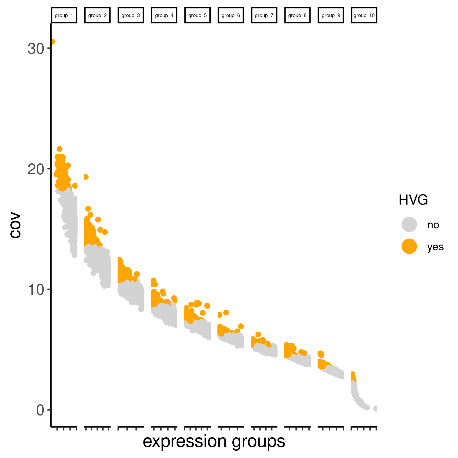
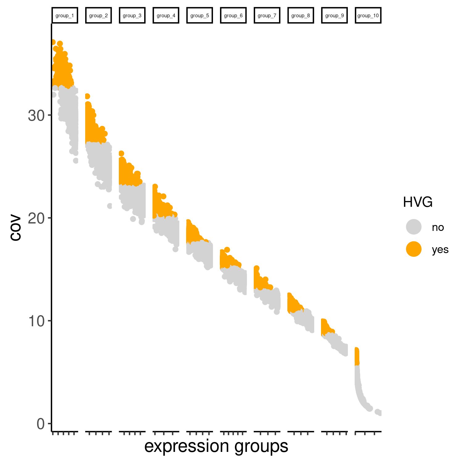
cere_rnaseq <- calculateHVG(gobject = cere_rnaseq, method = 'cov_groups', zscore_threshold = 0.5, nr_expression_groups = 10, reverse_log_scale=F, save_param = list(save_name="3_a_HVGplot", base_height=5, base_width=5))
gene_metadata = fDataDT(cere_rnaseq)
featgenes = gene_metadata[hvg == 'yes']$gene_ID
cere_rnaseq <- runPCA(gobject = cere_rnaseq, expression_values = 'custom', genes_to_use = featgenes, scale_unit = F, method="factominer", center=T)
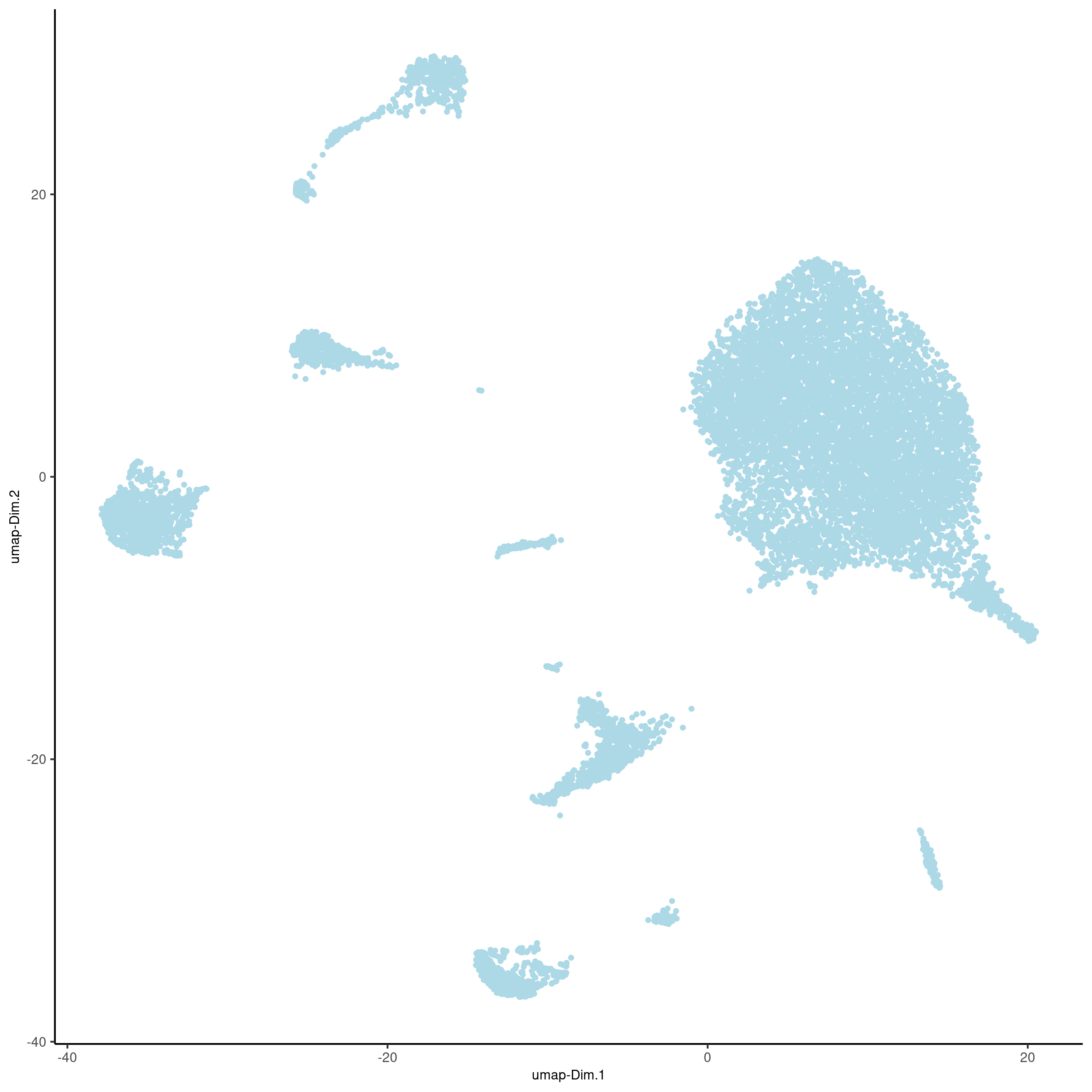
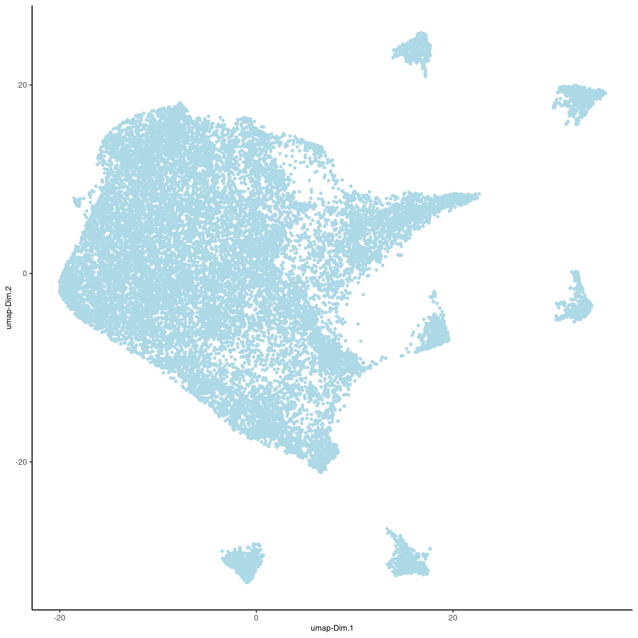
cere_rnaseq <- runUMAP(cere_rnaseq, dimensions_to_use=1:25, n_components=2)
plotUMAP(gobject=cere_rnaseq, point_size=1, save_param = list(save_name = '3_c_UMAP_reduction'))
cere_rnaseq<-createNearestNetwork(gobject=cere_rnaseq, dimensions_to_use=1:25, k=25)
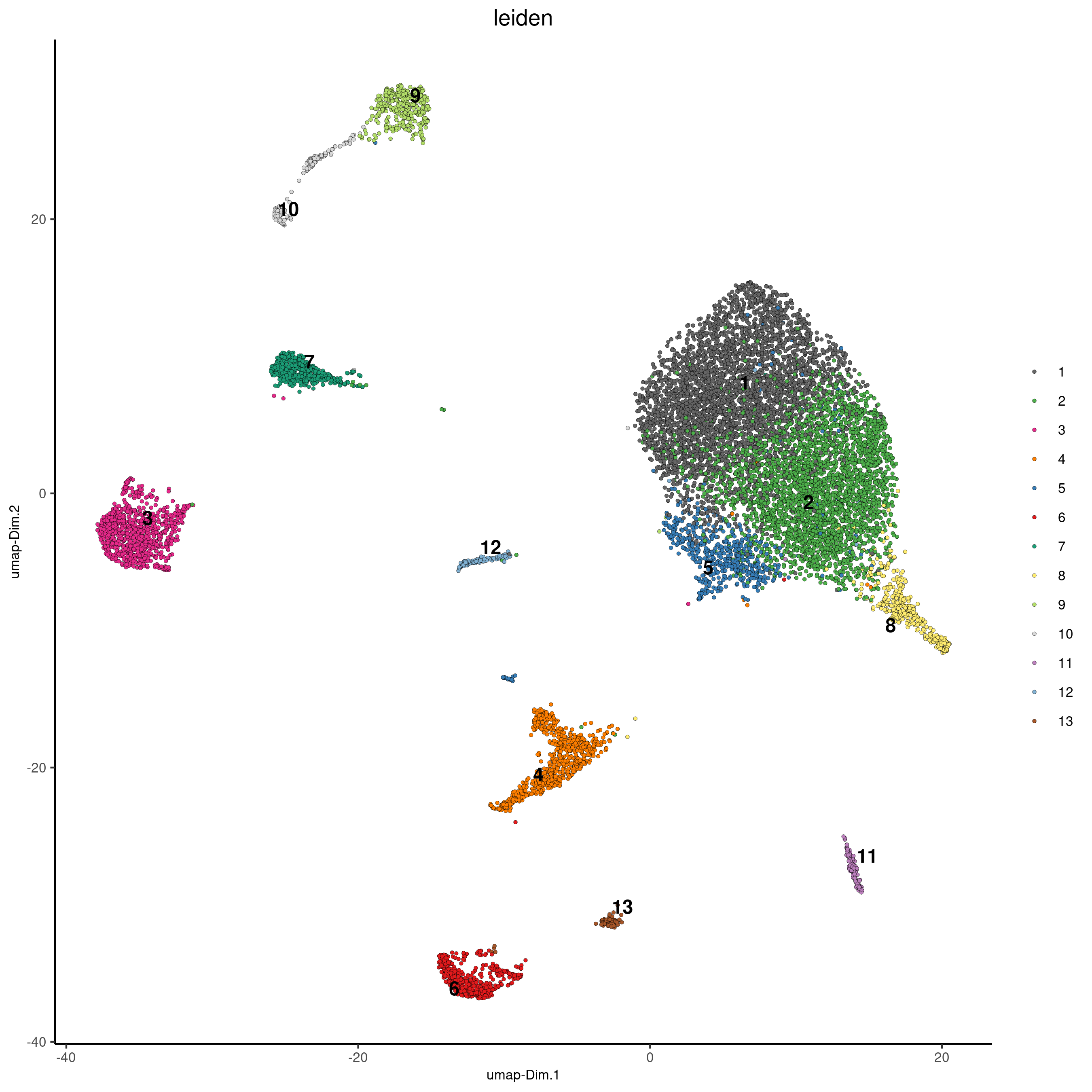
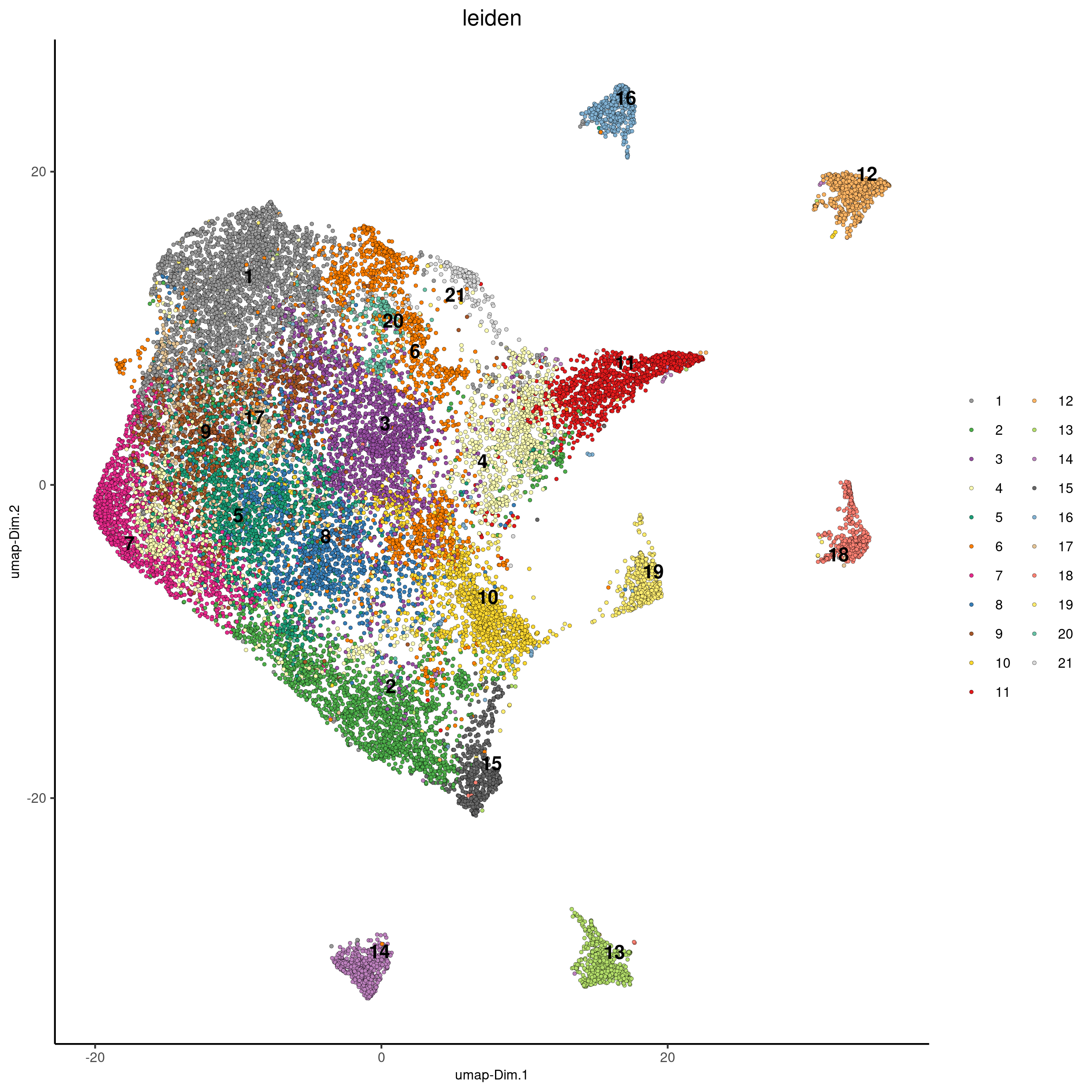
cere_rnaseq<-doLeidenCluster(gobject=cere_rnaseq, resolution=0.75, n_iterations=200, name="leiden")
plotUMAP(cere_rnaseq, cell_color="leiden", point_size=1, save_param = list(save_name = '4_a_UMAP_leiden'))

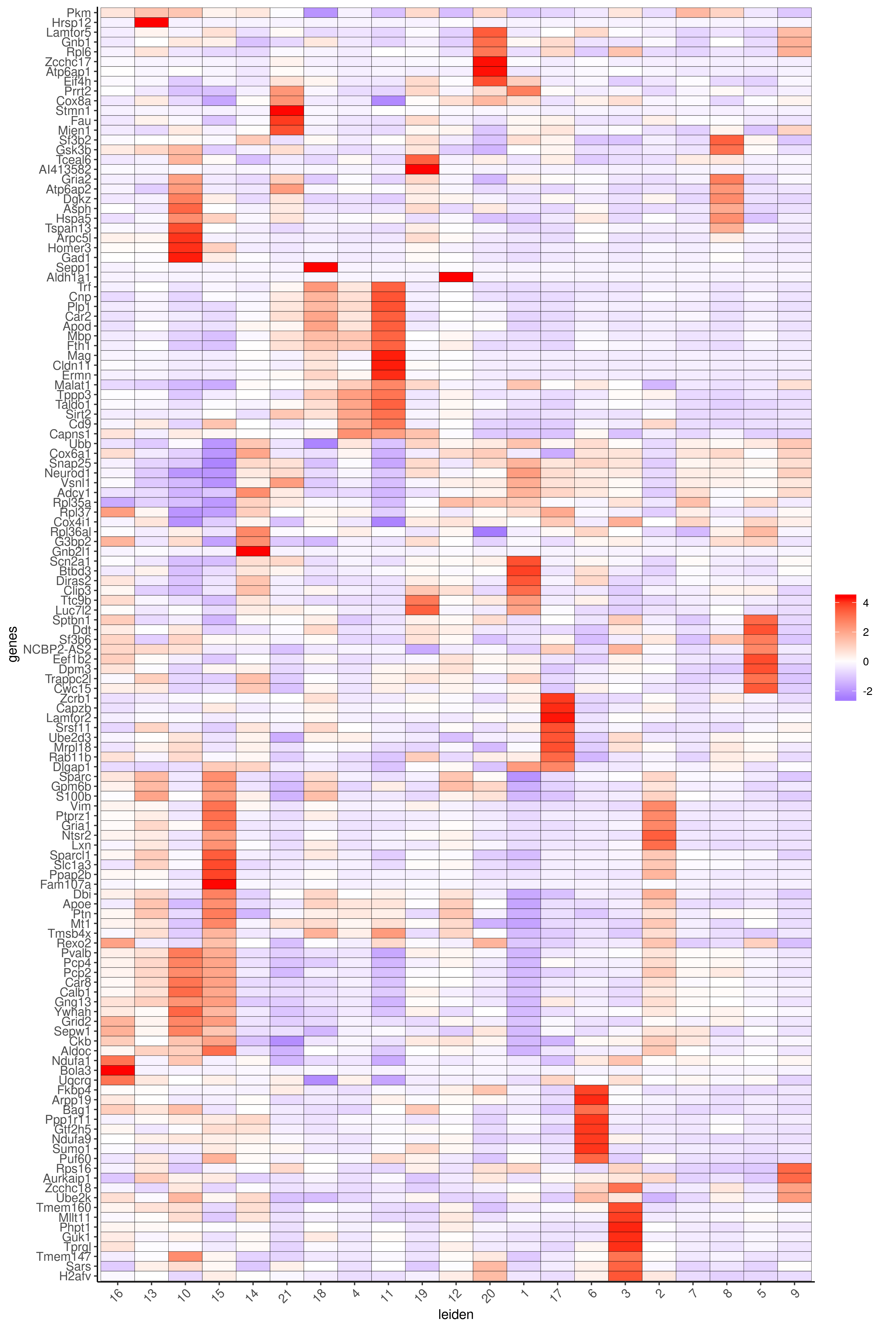
2.3. Identification of marker genes for cell types

library(scran)
markers_scarn=findMarkers_one_vs_all(gobject=cere_rnaseq, method="scran", expression_values="custom", cluster_column="leiden", min_genes=5)
markergenes_scran = unique(markers_scarn[, head(.SD, 8), by="cluster"][["genes"]])
plotMetaDataHeatmap(cere_rnaseq, expression_values="custom", metadata_cols=c("leiden"), selected_genes=markergenes_scran, save_param = c(save_name = '6_b_metaheatmap_scran'))

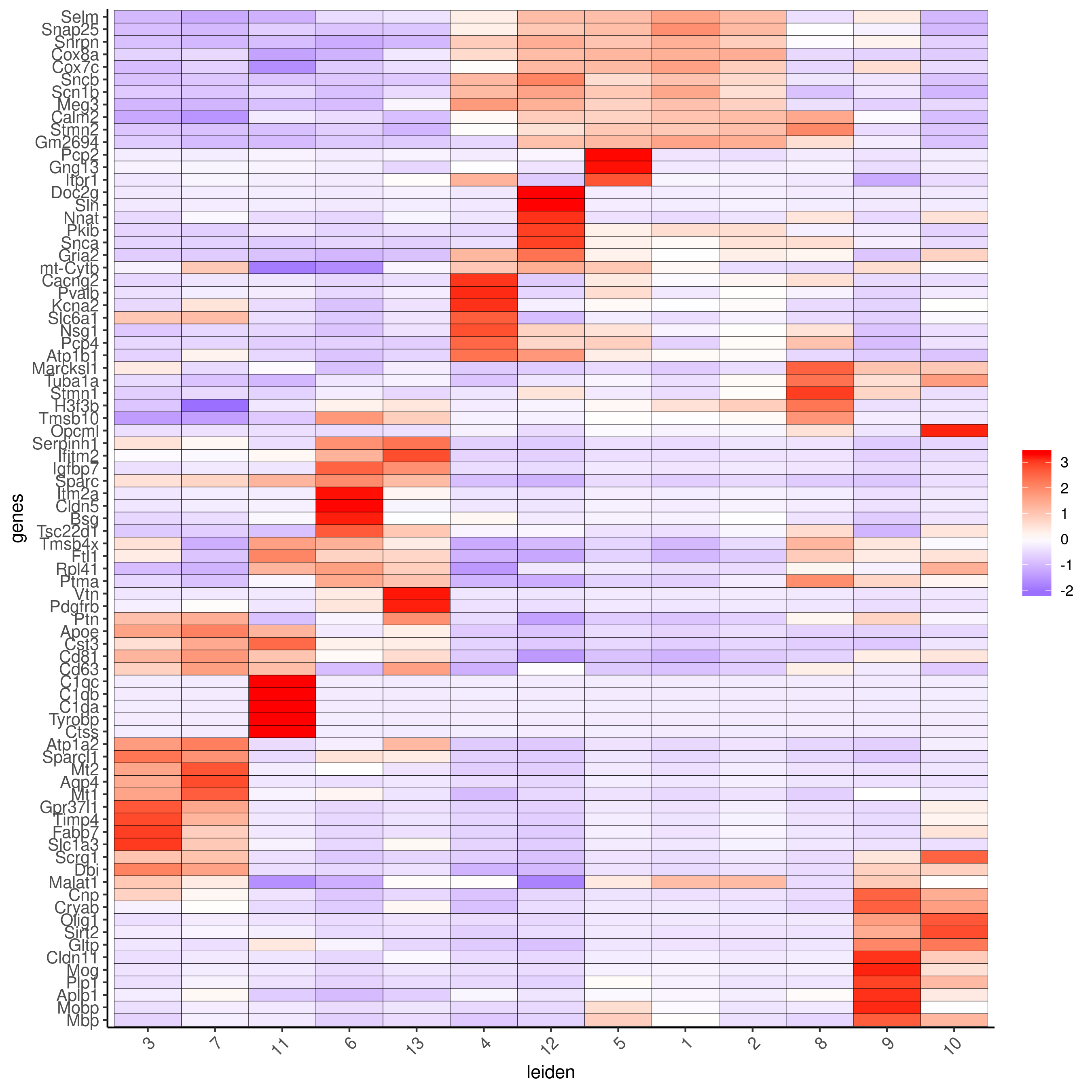
Legend: 4: GABAergic interneuron, 6: endothelial cells 1, 13: endothelial cells 2, 11: microglia/macrophages, 3,7: astrocyte-1 and astrocyte-2 or Bergmann Glia, 12: unipolar brush neurons, 1,2: neurons (granule), 5: Punkinje cells, 8: Golgi cells, 9: oligodendrocytes, 10: OPC

3. Processing and analyses of Slide-seq dataset

We download the cerebellum Slide-seq dataset from Broad institute single-cell portal.

3.1. Dataset loading

bead_positions <- data.table::fread(file=fs::path(my_working_dir, "BeadLocationsForR.csv"))
expr_matrix<-data.table::fread(file=fs::path(my_working_dir, "MappedDGEForR.csv"))
expr_mat = as.matrix(expr_matrix[,-1]);rownames(expr_mat) = expr_matrix$Row
Slide_test <- createGiottoObject(raw_exprs = expr_mat, spatial_locs = bead_positions[,.(xcoord, ycoord)], instructions=myinst)
filterCombinations(Slide_test, expression_thresholds = c(1, 1), gene_det_in_min_cells = c(20, 20, 20), min_det_genes_per_cell = c(20, 32, 100))
Slide_test<-filterGiotto(gobject=Slide_test, gene_det_in_min_cells=20, min_det_genes_per_cell=20)
non_mito_genes = grep(pattern = 'mt-', Slide_test@gene_ID, value = T, invert = T)
non_mito_or_blood_genes = grep(pattern = 'Hb[ab]', non_mito_genes, value = T, invert = T)
Slide_test = subsetGiotto(gobject = Slide_test, gene_ids = non_mito_or_blood_genes)
spatPlot(Slide_test, point_size=0.5)
Slide_test <- normalizeGiotto(gobject = Slide_test, scalefactor = 2000, verbose = T)
Slide_test <- addStatistics(gobject = Slide_test)
Slide_test <- calculateHVG(gobject = Slide_test, method = 'cov_groups', zscore_threshold = 0.5, nr_expression_groups = 10, save_param=list(save_name="slideseq_HVGplot", base_height=5, base_width=5))
gene_metadata = fDataDT(Slide_test)
featgenes = gene_metadata[hvg == 'yes']$gene_ID

3.2. PCA, UMAP, and clustering

Slide_test <- adjustGiottoMatrix(gobject = Slide_test, expression_values = c('normalized'), batch_columns = NULL, covariate_columns = c('nr_genes', 'total_expr'),  return_gobject = TRUE, update_slot = c('custom'))
Slide_test <- runPCA(gobject = Slide_test, expression_values = 'custom', genes_to_use = featgenes, scale_unit = F, center=T, method="factominer")
Giotto::plotPCA(gobject=Slide_test)
Slide_test <- runUMAP(Slide_test, dimensions_to_use=1:9, n_components=2)
plotUMAP(gobject=Slide_test, point_size=1, save_param = list(save_name = 'slideseq_UMAP'))
Slide_test<-createNearestNetwork(gobject=Slide_test, dimensions_to_use=1:9, k=20)
Slide_test<-doLeidenCluster(gobject=Slide_test, resolution=0.6, n_iterations=10, name="leiden")
plotUMAP(gobject=Slide_test, cell_color="leiden", point_size=1, save_param = list(save_name = 'slideseq_UMAP_leiden'))
markers_scarn=findMarkers_one_vs_all(gobject=Slide_test, method="scran", expression_values="custom", cluster_column="leiden", min_genes=5)
markergenes_scran = unique(markers_scarn[, head(.SD, 8), by="cluster"][["genes"]])
plotMetaDataHeatmap(Slide_test, expression_values="custom", metadata_cols=c("leiden"), selected_genes=markergenes_scran, save_param = c(save_name = 'slideseq_metaheatmap_scran'))

3. Integrative analysis of scRNAseq and slideSeq

3.1. Cell type enrichment analysis (RANK method)

This is the main section. We first intersect the two datasets to find common genes. Then we define the rank signature matrix (genes by cell types) on the scRNAseq dataset. We call the runRankEnrich function to perform the enrichment analysis.

common_genes=intersect(rownames(cere_rnaseq@raw_exprs), rownames(Slide_test@raw_exprs))
cere_rnaseq2 = subsetGiotto(cere_rnaseq, gene_ids = common_genes)
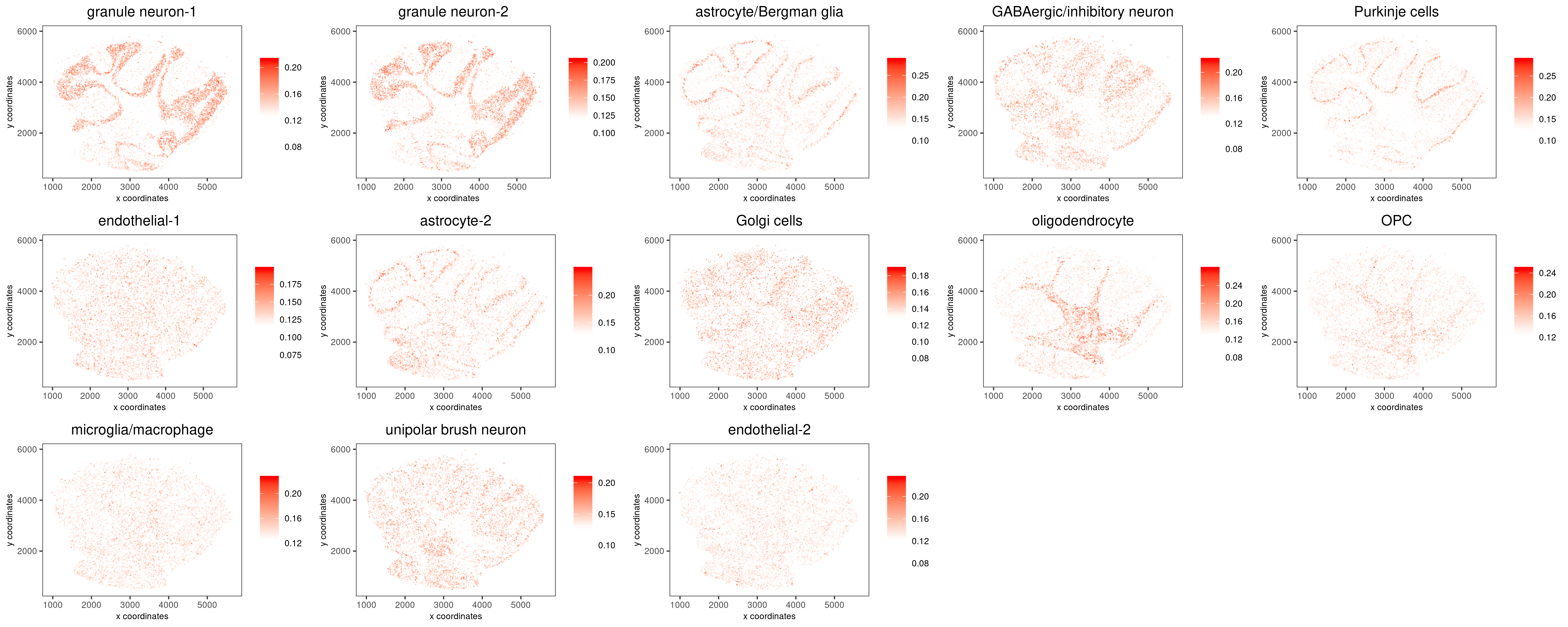
annot=c("granule neuron-1", "granule neuron-2", "astrocyte/Bergman glia", "GABAergic/inhibitory neuron", "Purkinje cells", "endothelial-1", "astrocyte-2", "Golgi cells", "oligodendrocyte", "OPC", "microglia/macrophage", "unipolar brush neuron", "endothelial-2")
rank_matrix=makeSignMatrixRank(sc_matrix=cere_rnaseq2@raw_exprs, sc_cluster_ids=pDataDT(cere_rnaseq2)$leiden, ties.method="random")
Slide_test<-runRankEnrich(Slide_test, sign_matrix=rank_matrix, expression_values="norm", reverse_log_scale=F, logbase=2, output_enrichment="original", name="rank", rbp_p=0.99, num_agg=100, ties.method="random")
colnames(Slide_test@spatial_enrichment$rank) <- c("cell_ID", annot)
spatCellPlot(gobject = Slide_test, spat_enr_names = 'rank', cell_annotation_values = annot, cow_n_col = 5, coord_fix_ratio = NULL, point_size=0.5, point_border_stroke=0, cell_color_gradient=c("white", "white", "red"), save_param=c(save_name="rank", base_width=20, base_height=8))