STARmap dataset

0. Environment

library(Giotto)
# STOP!
# ====== 1. set working directory ======
# For Docker, set my_working_dir to /data
my_working_dir = '/data'
# For native install users, set my_working_dir to a directory accessible by user
#my_working_dir = "/home/qzhu/Downloads"
# ====== 2. set giotto python path ======
# For Docker, set python_path to /usr/bin/python3
python_path = "/usr/bin/python3"
# For native install users, python path may be different, and may depend on whether conda or virtual environment. One can check by "reticulate::py_discover_config()" to see which python is picked up automatically. Then set python_path to what is returned by py_discover_config.
# python_path = "/usr/bin/python3"

1. Dataset preparation steps

1.1. Dataset explanation

Wang et al. created a 3D spatial expression dataset consisting of 28 genes from 32,845 single cells in a visual cortex volume using the STARmap technology.

The STARmap data to run this tutorial can be found here. Alternatively you can use the getSpatialDataset to automatically download this dataset like we do in this example.

1.2. Dataset download

# download data to working directory
# if wget is installed, set method = 'wget'
getSpatialDataset(dataset = 'starmap_3D_cortex', directory = my_working_dir, method = 'wget')

1.3. Giotto global instructions and preparations

## instructions allow us to automatically save all plots into a chosen results folder
instrs = createGiottoInstructions(show_plot = FALSE,save_plot = TRUE, save_dir = my_working_dir,python_path = python_path)
expr_path = fs::path(my_working_dir, "STARmap_3D_data_expression.txt")
loc_path = fs::path(my_working_dir, "STARmap_3D_data_cell_locations.txt")

2. Create Giotto object & process data

## create
STAR_test <- createGiottoObject(raw_exprs = expr_path,spatial_locs = loc_path,instructions = instrs)
## filter raw data
# pre-test filter parameters
filterDistributions(STAR_test, detection = 'genes',save_param = list(save_name = '2_a_distribution_genes'))

filterDistributions(STAR_test, detection = 'cells',save_param = list(save_name = '2_b_distribution_cells'))

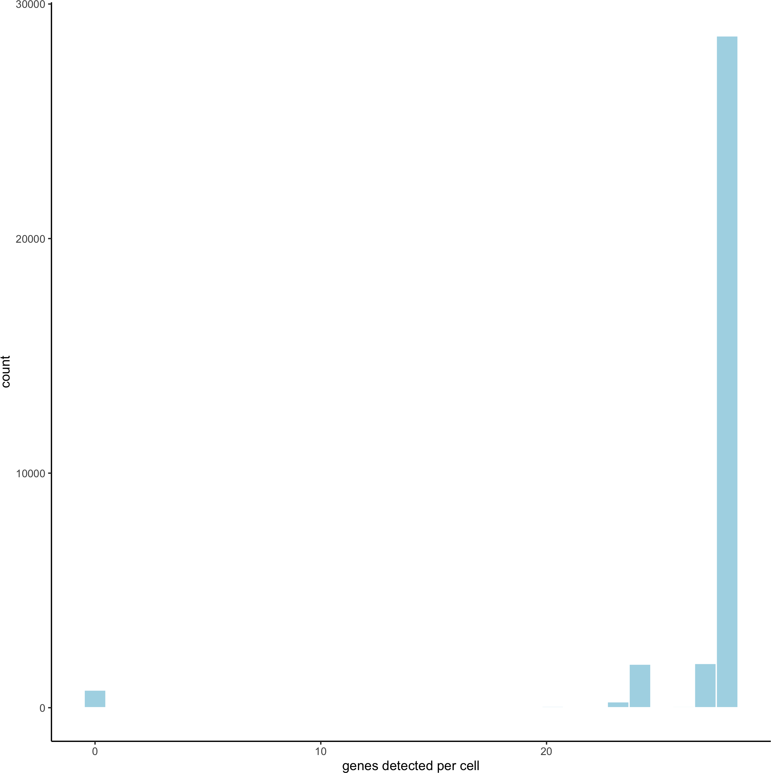
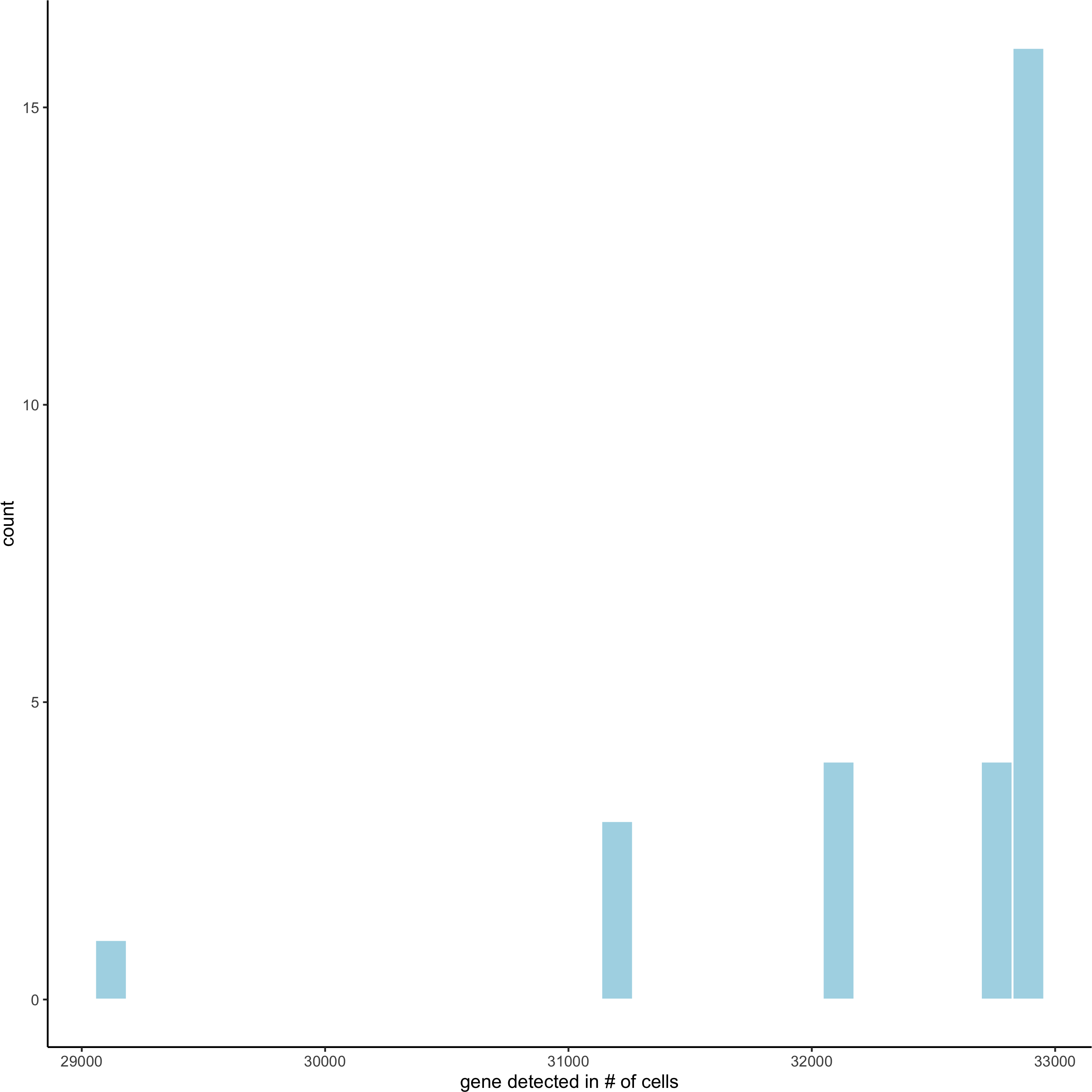
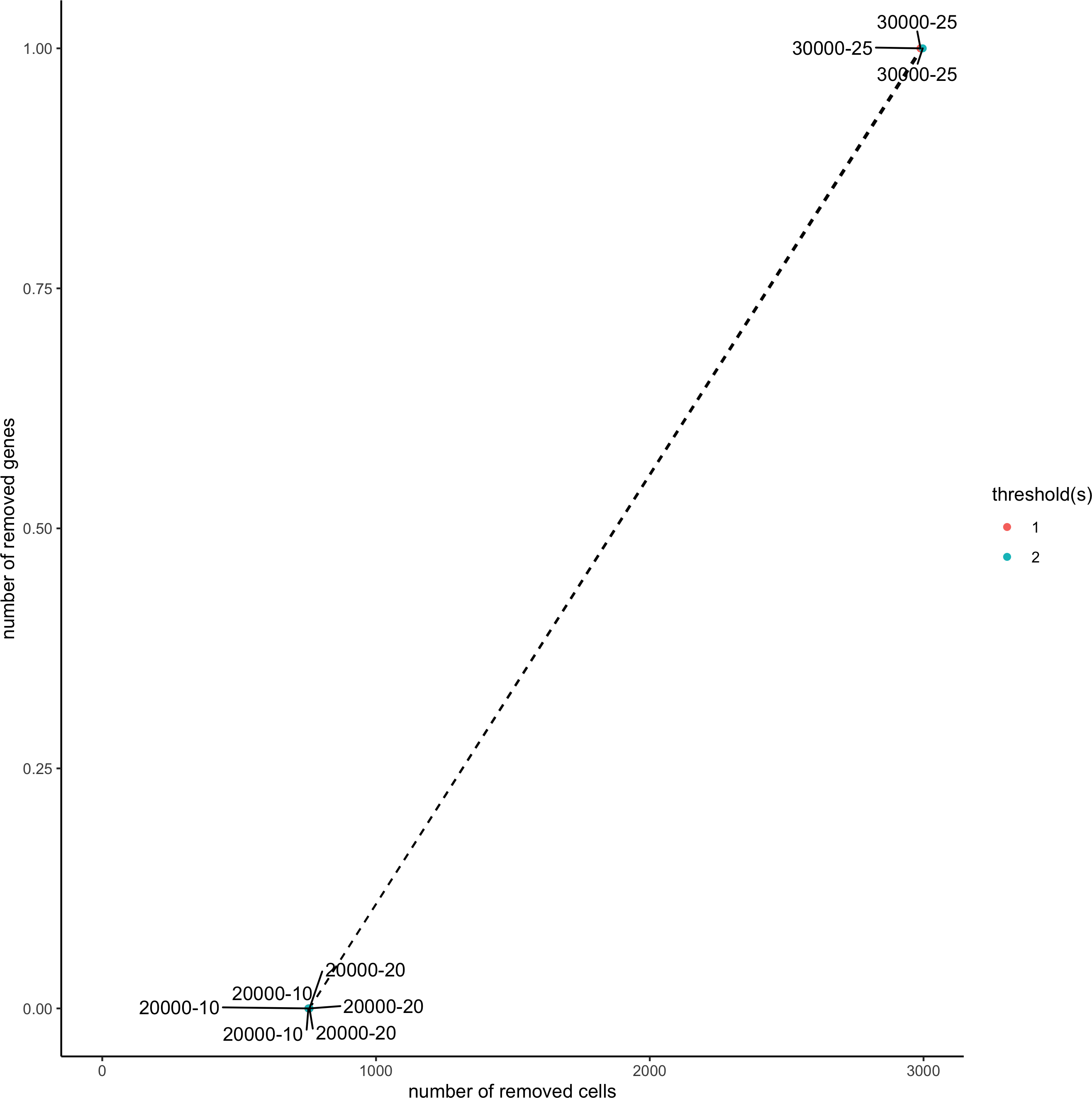
filterCombinations(STAR_test, expression_thresholds = c(1, 1,2),gene_det_in_min_cells = c(20000, 20000, 30000),min_det_genes_per_cell = c(10, 20, 25),save_param = list(save_name = '2_c_distribution_filters'))

# filter
STAR_test <- filterGiotto(gobject = STAR_test,gene_det_in_min_cells = 20000,min_det_genes_per_cell = 20)
## normalize
STAR_test <- normalizeGiotto(gobject = STAR_test, scalefactor = 10000, verbose = T)
STAR_test <- addStatistics(gobject = STAR_test)
STAR_test <- adjustGiottoMatrix(gobject = STAR_test, expression_values = c('normalized'),batch_columns = NULL, covariate_columns = c('nr_genes', 'total_expr'),return_gobject = TRUE,update_slot = c('custom'))
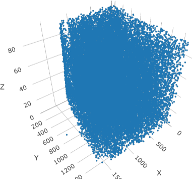
## visualize
# 3D
spatPlot3D(gobject = STAR_test, point_size = 2,save_param = list(save_name = '2_d_spatplot_3D'))

3. Dimension reduction

STAR_test <- calculateHVG(gobject = STAR_test, method = 'cov_groups', 
zscore_threshold = 0.5, nr_expression_groups = 3,save_param = list(save_name = '3_a_HVGplot', base_height = 5, base_width = 5))

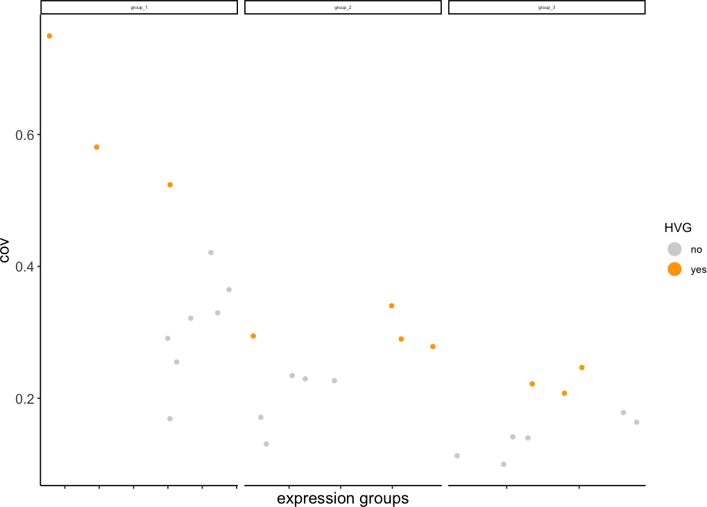
# too few highly variable genes
# genes_to_use = NULL is the default and will use all genes available
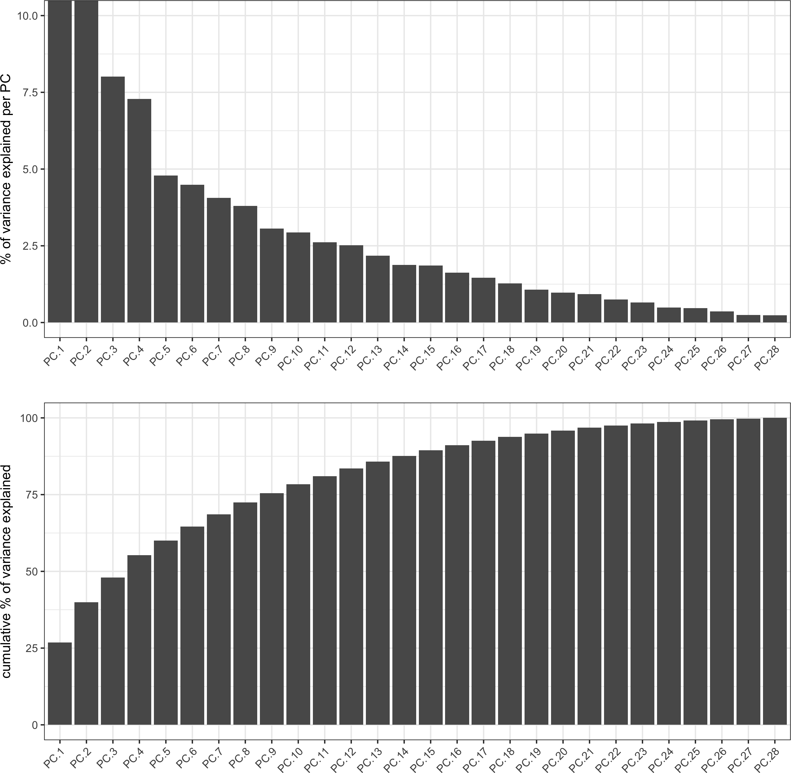
STAR_test <- runPCA(gobject = STAR_test, genes_to_use = NULL, scale_unit = F,method = 'factominer')
signPCA(STAR_test,save_param = list(save_name = '3_b_signPCs'))

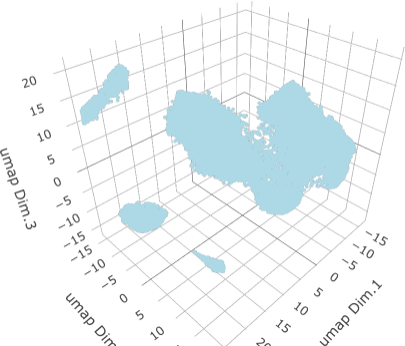
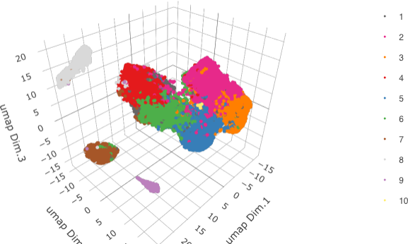
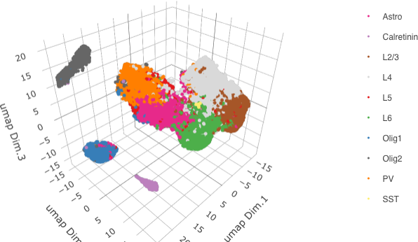
STAR_test <- runUMAP(STAR_test, dimensions_to_use = 1:8, n_components = 3, n_threads = 4)
plotUMAP_3D(gobject = STAR_test,save_param = list(save_name = '3_c_UMAP'))

4. Cluster

## sNN network (default)
STAR_test <- createNearestNetwork(gobject = STAR_test, dimensions_to_use = 1:8, k = 15)
## Leiden clustering
STAR_test <- doLeidenCluster(gobject = STAR_test, resolution = 0.2, n_iterations = 100,name = 'leiden_0.2')
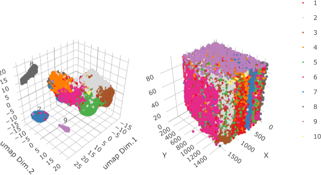
plotUMAP_3D(gobject = STAR_test, cell_color = 'leiden_0.2',show_center_label = F,save_param = list(save_name = '4_a_UMAP'))

5. Co-visualize

spatDimPlot3D(gobject = STAR_test,cell_color = 'leiden_0.2',save_param = list(save_name = '5_a_spatDimPlot'))

6. Differential expression

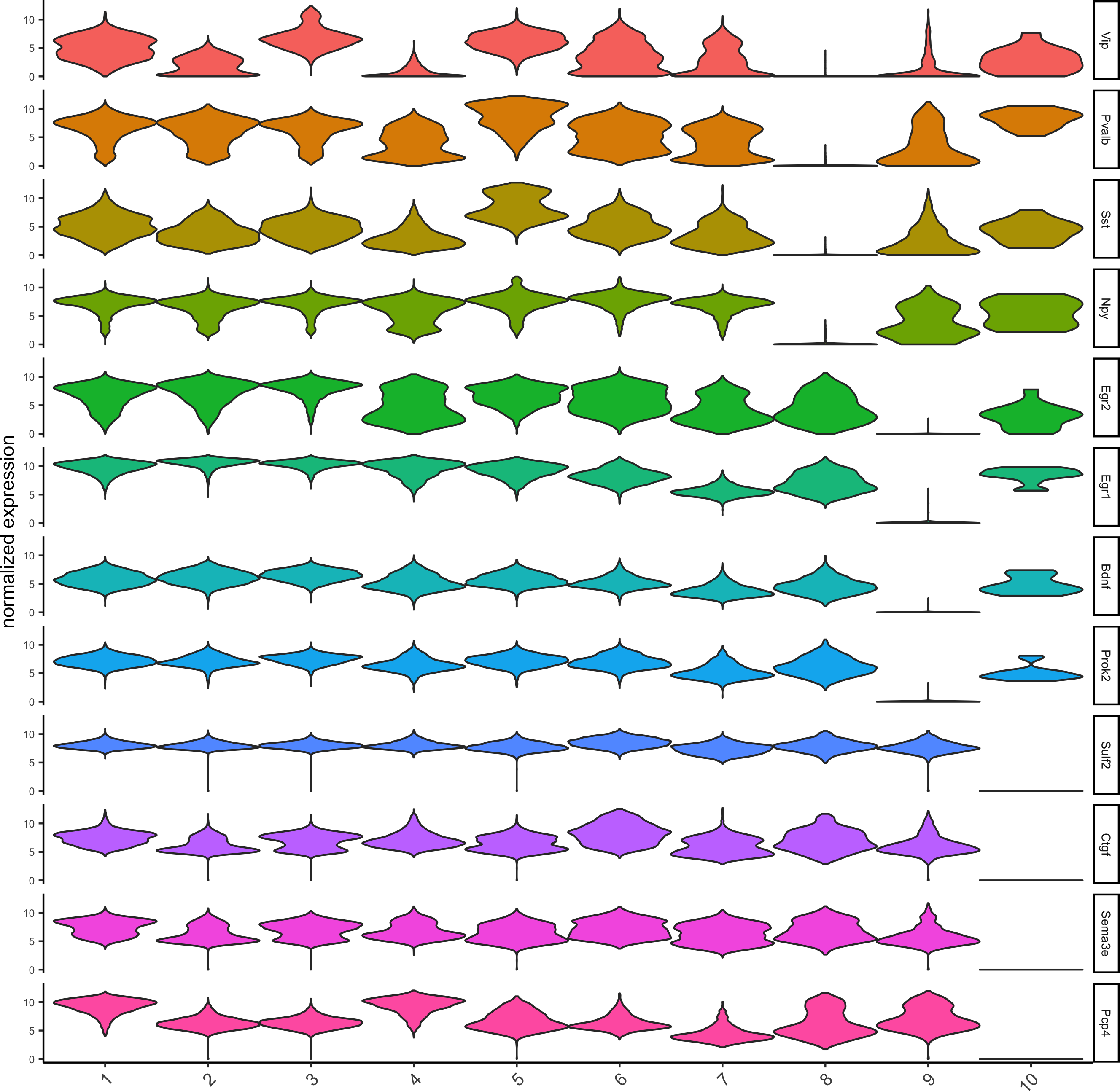
markers = findMarkers_one_vs_all(gobject = STAR_test,method = 'gini',expression_values = 'normalized',cluster_column = 'leiden_0.2',min_expr_gini_score = 2,min_det_gini_score = 2,min_genes = 5, rank_score = 2)
markers[, head(.SD, 2), by = 'cluster']
# violinplot
violinPlot(STAR_test, genes = unique(markers$genes), cluster_column = 'leiden_0.2',strip_position = "right", save_param = list(save_name = '6_a_violinplot'))

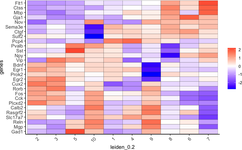
# cluster heatmap
plotMetaDataHeatmap(STAR_test, expression_values = 'scaled',metadata_cols = c('leiden_0.2'),save_param = list(save_name = '6_b_metaheatmap'))

7. Cell-type annotation

## general cell types
clusters_cell_types_cortex = c('excit','excit','excit', 'inh', 'excit','other', 'other', 'other', 'inh', 'inh')
names(clusters_cell_types_cortex) = c(1:10)
STAR_test = annotateGiotto(gobject = STAR_test, annotation_vector = clusters_cell_types_cortex,cluster_column = 'leiden_0.2', name = 'general_cell_types')
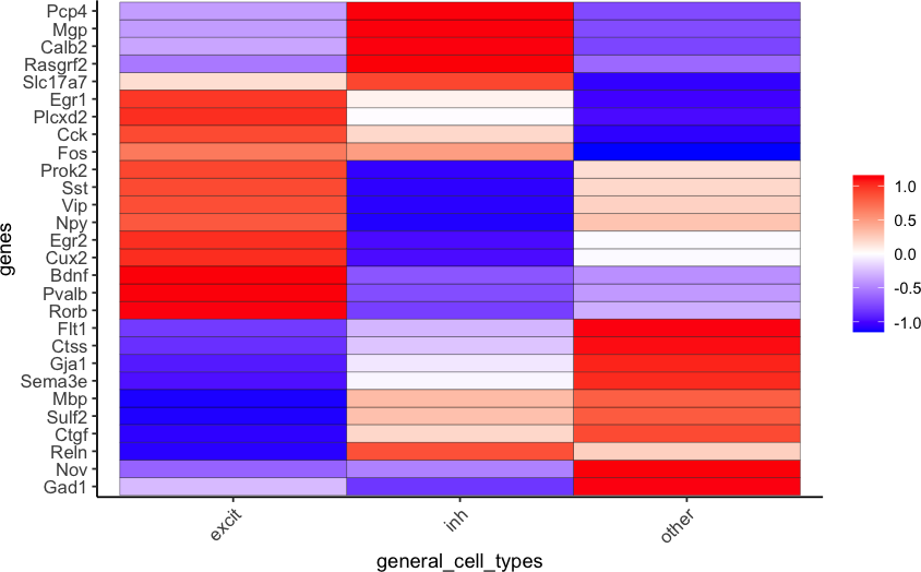
plotMetaDataHeatmap(STAR_test, expression_values = 'scaled',metadata_cols = c('general_cell_types'),save_param = list(save_name = '7_a_metaheatmap'))

## detailed cell types
clusters_cell_types_cortex = c('L5','L4','L2/3', 'PV', 'L6','Astro', 'Olig1', 'Olig2', 'Calretinin', 'SST')
names(clusters_cell_types_cortex) = c(1:10)
STAR_test = annotateGiotto(gobject = STAR_test, annotation_vector = clusters_cell_types_cortex,cluster_column = 'leiden_0.2', name = 'cell_types')
plotUMAP_3D(STAR_test, cell_color = 'cell_types', point_size = 1.5,show_center_label = F,save_param = list(save_name = '7_b_UMAP'))

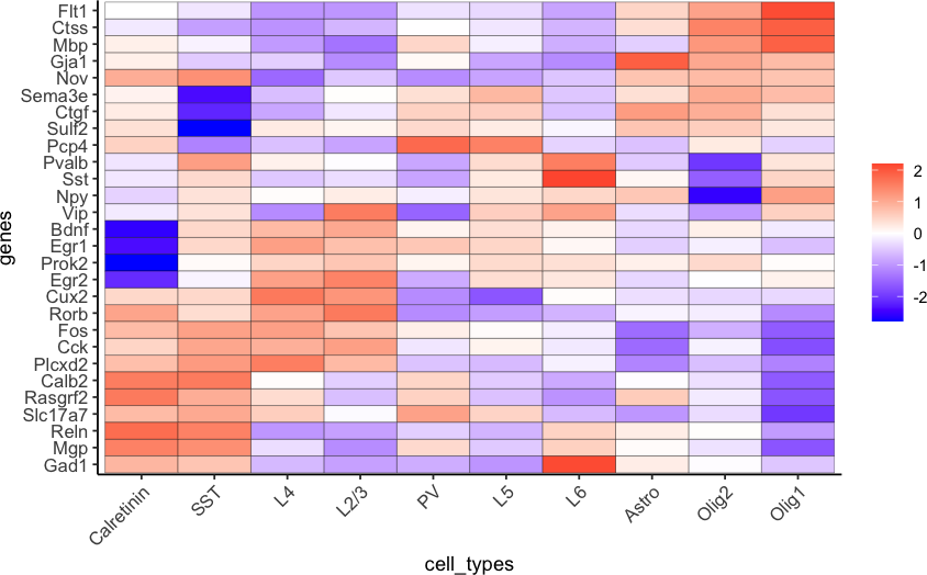
plotMetaDataHeatmap(STAR_test, expression_values = 'scaled',metadata_cols = c('cell_types'),custom_cluster_order = c("Calretinin", "SST", "L4", "L2/3", "PV", "L5", "L6", "Astro", "Olig2", "Olig1"),save_param = list(save_name = '7_c_metaheatmap'))

8. Co-visualize cell types

# create consistent color code
mynames = unique(pDataDT(STAR_test)$cell_types)
mycolorcode = Giotto:::getDistinctColors(n = length(mynames))
names(mycolorcode) = mynames
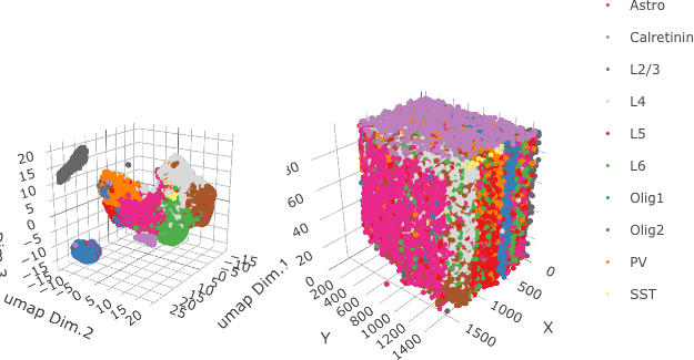
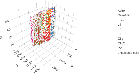
spatDimPlot3D(gobject = STAR_test,cell_color = 'cell_types',show_center_label = F,save_param = list(save_name = '8_a_spatdimplot'))

9. Visualize gene expression

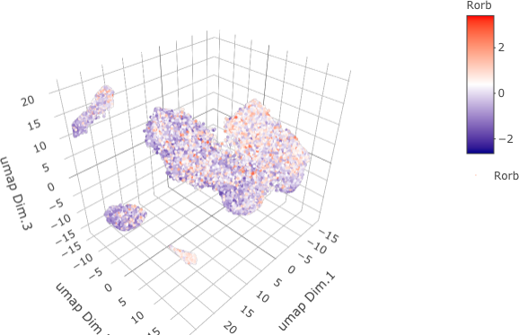
dimGenePlot3D(STAR_test, expression_values = 'scaled',genes = "Rorb",genes_high_color = 'red', genes_mid_color = 'white', genes_low_color = 'darkblue',save_param = list(save_name = '9_a_dimGenePlot'))

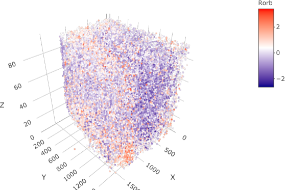
spatGenePlot3D(STAR_test, 
expression_values = 'scaled',genes = "Rorb",show_other_cells = F,genes_high_color = 'red', genes_mid_color = 'white', genes_low_color = 'darkblue',save_param = list(save_name = '9_b_spatGenePlot'))

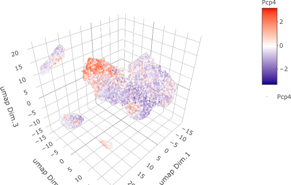
dimGenePlot3D(STAR_test, expression_values = 'scaled',genes = "Pcp4",genes_high_color = 'red', genes_mid_color = 'white', genes_low_color = 'darkblue',save_param = list(save_name = '9_c_dimGenePlot'))

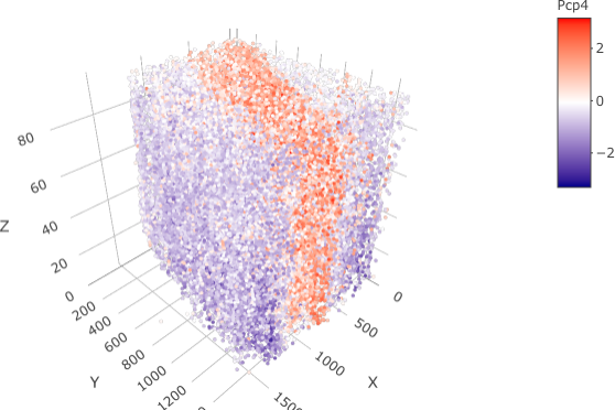
spatGenePlot3D(STAR_test, 
expression_values = 'scaled',genes = "Pcp4",show_other_cells = F,genes_high_color = 'red', genes_mid_color = 'white', genes_low_color = 'darkblue',save_param = list(save_name = '9_d_spatGenePlot'))

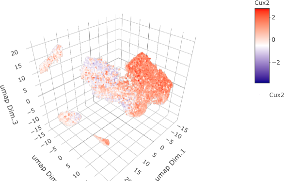
dimGenePlot3D(STAR_test, expression_values = 'scaled',genes = "Cux2",genes_high_color = 'red', genes_mid_color = 'white', genes_low_color = 'darkblue',save_param = list(save_name = '9_e_dimGenePlot'))

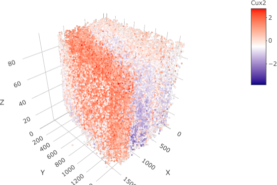
spatGenePlot3D(STAR_test, 
expression_values = 'scaled',genes = "Cux2",show_other_cells = F,genes_high_color = 'red', genes_mid_color = 'white', genes_low_color = 'darkblue',save_param = list(save_name = '9_f_spatGenePlot'))

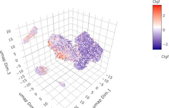
dimGenePlot3D(STAR_test, expression_values = 'scaled',genes = "Ctgf",genes_high_color = 'red', genes_mid_color = 'white', genes_low_color = 'darkblue',save_param = list(save_name = '9_g_dimGenePlot'))

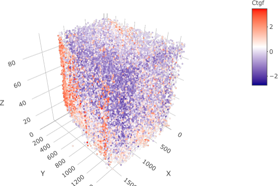
spatGenePlot3D(STAR_test, 
expression_values = 'scaled',genes = "Ctgf",show_other_cells = F,genes_high_color = 'red', genes_mid_color = 'white', genes_low_color = 'darkblue',save_param = list(save_name = '9_h_spatGenePlot'))

10. Virtual cross section

STAR_test <- createSpatialNetwork(gobject = STAR_test, delaunay_method = 'delaunayn_geometry')
STAR_test = createCrossSection(STAR_test,method="equation",equation=c(0,1,0,600),extend_ratio = 0.6)

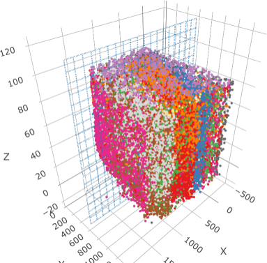
insertCrossSectionSpatPlot3D(STAR_test, cell_color = 'cell_types', axis_scale = 'cube',point_size = 2,cell_color_code = mycolorcode)

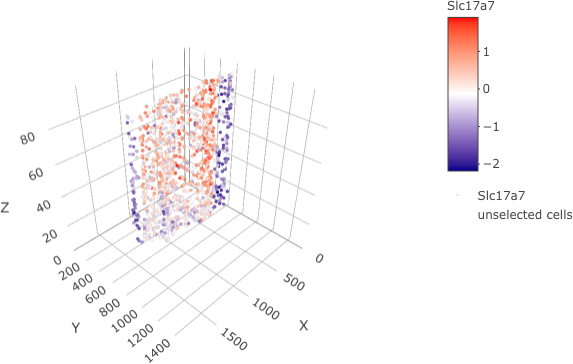
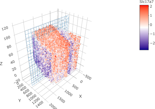
insertCrossSectionGenePlot3D(STAR_test, expression_values = 'scaled', axis_scale = "cube",genes = "Slc17a7")

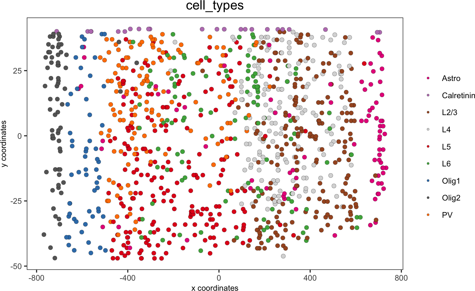
crossSectionPlot(STAR_test,point_size = 2, point_shape = "border",cell_color = "cell_types",cell_color_code = mycolorcode,save_param = list(save_name = '10_a_crossSectionPlot'))

crossSectionPlot3D(STAR_test,point_size = 2, cell_color = "cell_types", 
cell_color_code = mycolorcode,axis_scale = "cube",save_param = list(save_name = '10_b_crossSectionPlot3D'))

crossSectionGenePlot(STAR_test,genes = "Slc17a7",point_size = 2,point_shape = "border",cow_n_col = 1.5,expression_values = 'scaled',save_param = list(save_name = '10_c_crossSectionGenePlot'))

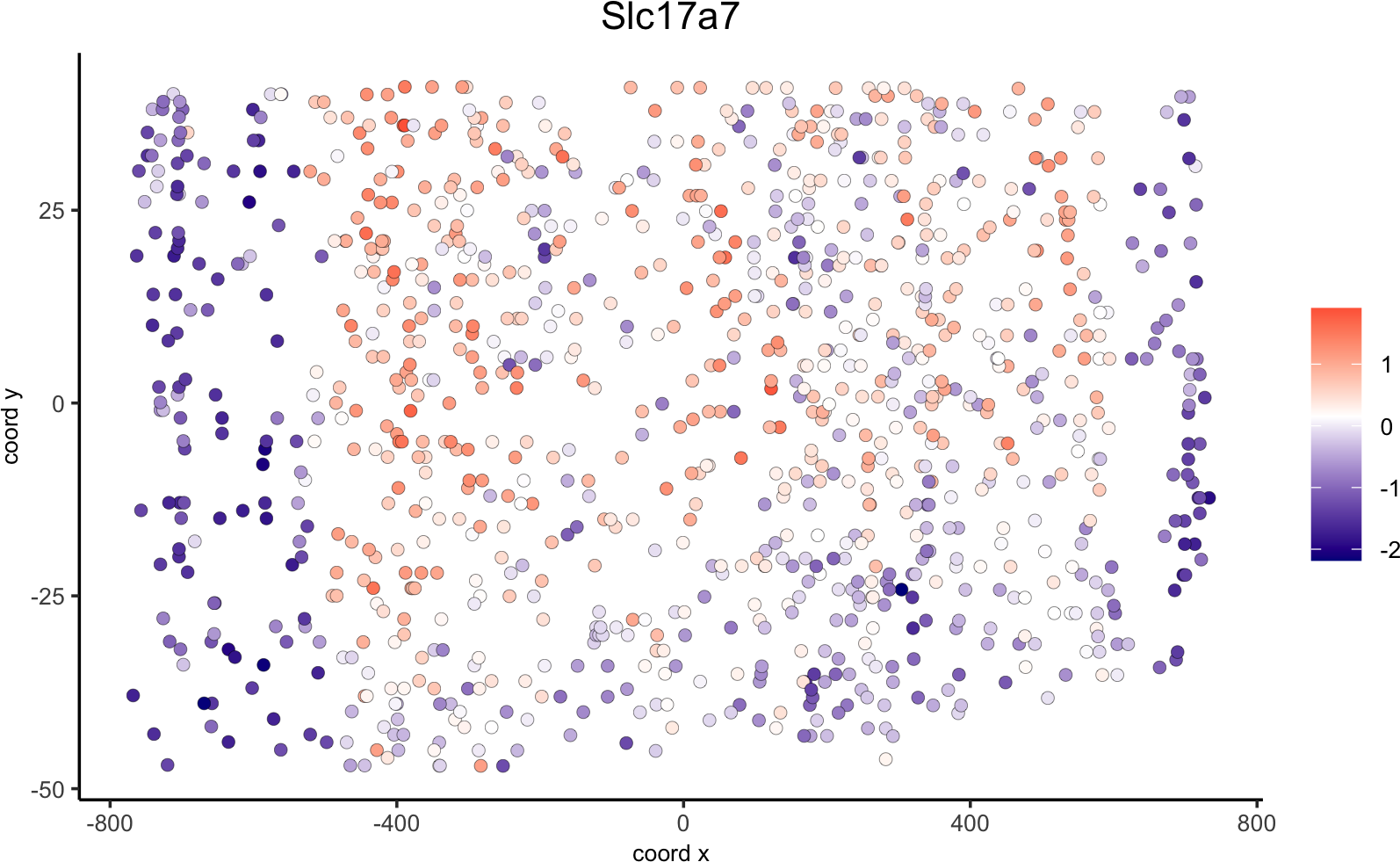
crossSectionGenePlot3D(STAR_test,point_size = 2,genes = c("Slc17a7"),expression_values = 'scaled',save_param = list(save_name = '10_d_crossSectionGenePlot3D'))