10X Visium brain dataset

1. Data input.

1.2. Dataset download

library(Giotto)
## provide path to visium folder
data_path = '/media/qzhu/My Passport/10x_visium_dset/mouse_brain_coronal/' #containing raw_feature_bc_matrix folder and spatial folder
workdir="/media/qzhu/My Passport/visium.example" #where results and plots will be saved
expr_data_path=fs::path(data_path, "raw_feature_bc_matrix")
raw_matrix=get10Xmatrix(path_to_data=expr_data_path, gene_column_index=2)
spatial_locations=data.table::fread(fs::path(data_path, "spatial", "tissue_positions_list.csv"))
spatial_locations = spatial_locations[match(colnames(raw_matrix), V1)]
colnames(spatial_locations) = c('barcode', 'in_tissue', 'array_row', 'array_col', 'col_pxl', 'row_pxl')
myinst=createGiottoInstructions(save_plot=T, show_plot=F, save_dir=workdir, python_path="/usr/bin/python3")

2. Create Giotto object & process data.

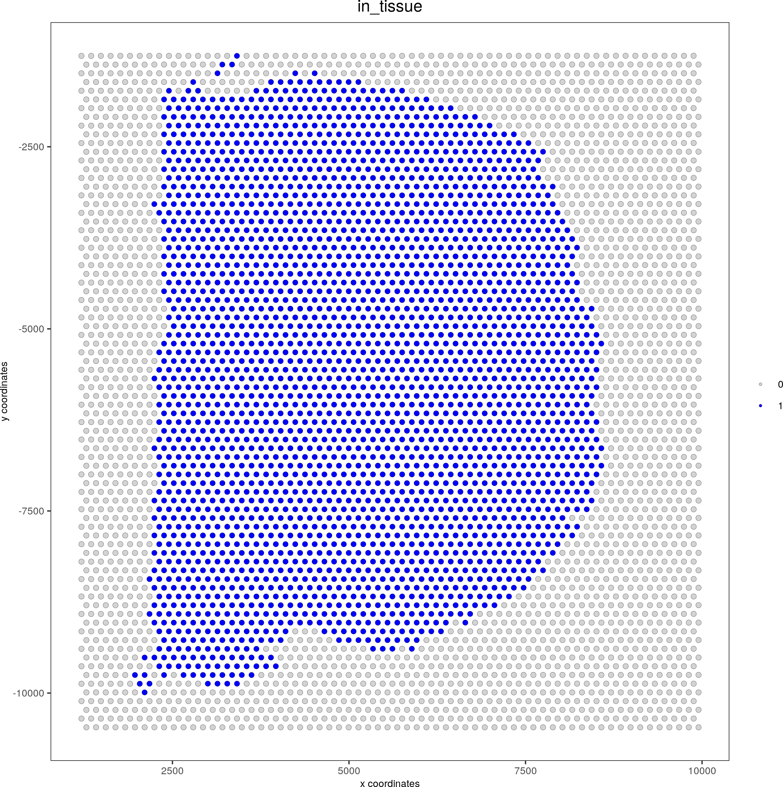
visium_brain <- createGiottoObject(raw_exprs = raw_matrix, spatial_locs = spatial_locations[,.(row_pxl,-col_pxl)], instructions = myinst, cell_metadata = spatial_locations[,.(in_tissue, array_row, array_col)])

spatPlot(gobject = visium_brain,  point_size = 2, cell_color = 'in_tissue', cell_color_code = c('0' = 'lightgrey', '1' = 'blue'), save_param=c(save_name="1-spatplot"))

metadata = pDataDT(visium_brain)
in_tissue_barcodes = metadata[in_tissue == 1]$cell_ID
visium_brain = subsetGiotto(visium_brain, cell_ids = in_tissue_barcodes)
## filter genes and cells
visium_brain <- filterGiotto(gobject = visium_brain, expression_threshold = 1,gene_det_in_min_cells = 50, min_det_genes_per_cell = 1000,expression_values = c('raw'),verbose = T)
## normalize
visium_brain <- normalizeGiotto(gobject = visium_brain, scalefactor = 6000, verbose = T)
## add gene & cell statistics
visium_brain <- addStatistics(gobject = visium_brain)
## visualize
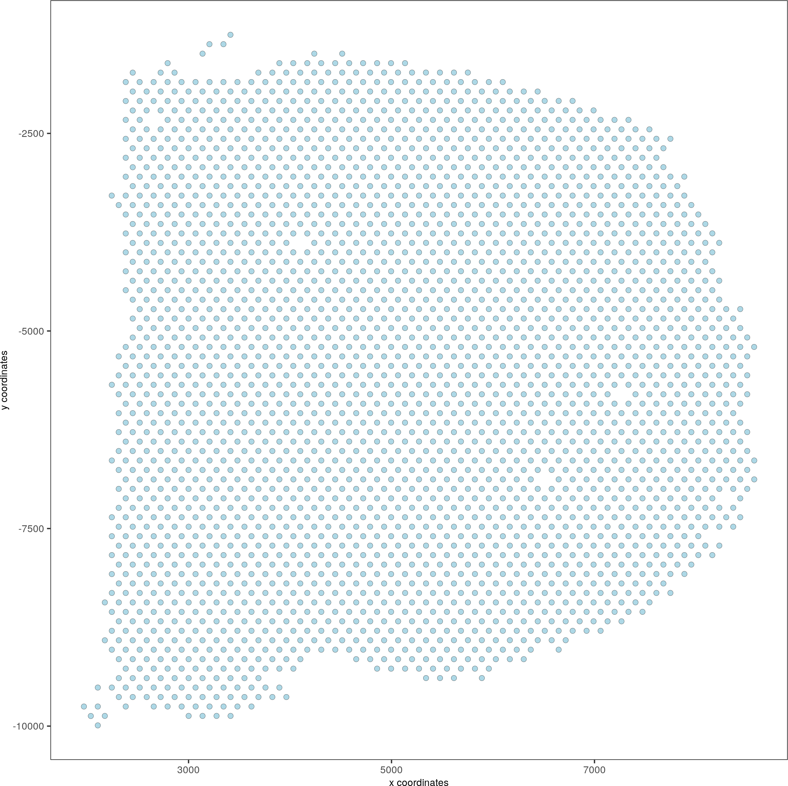
# location of spots
spatPlot(gobject = visium_brain,  point_size = 2, save_param=c(save_name="2-spatplot"))
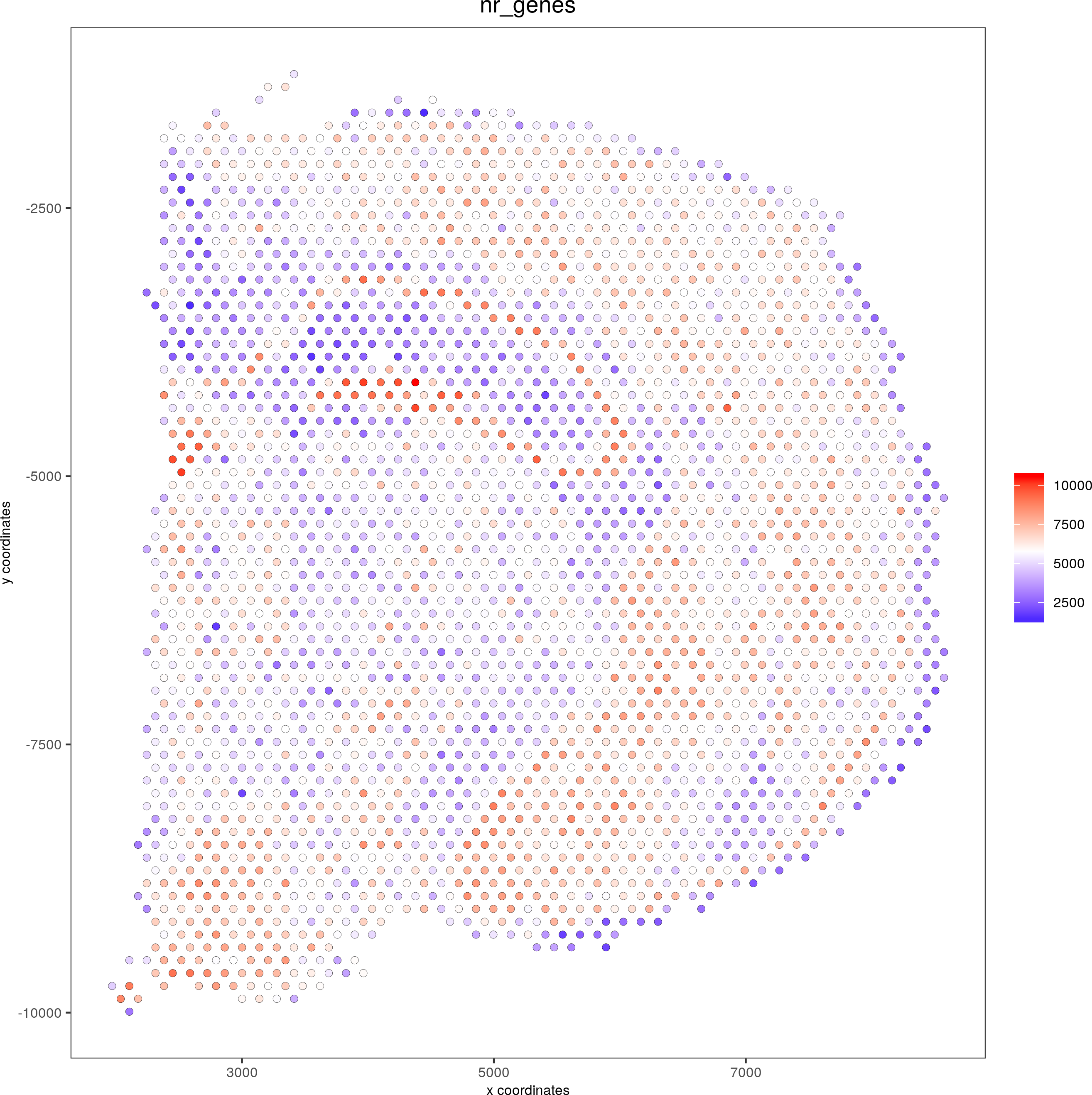
spatPlot(gobject = visium_brain, cell_color = 'nr_genes', color_as_factor = F,  point_size = 2, save_param=c(save_name="3-spatplot"))

3. Dimensional reduction

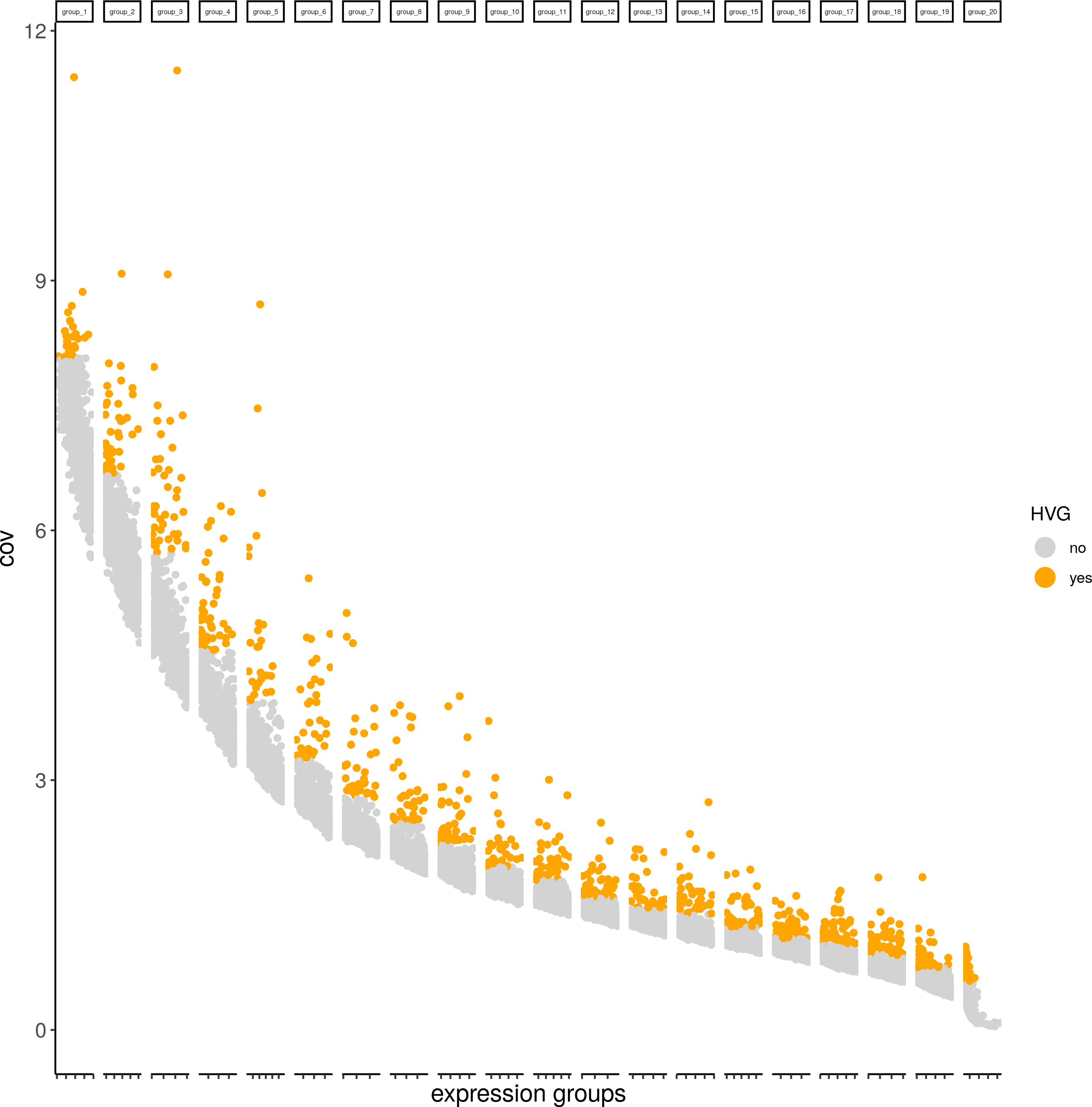
Highly variable genes

visium_brain <- calculateHVG(gobject = visium_brain)

PCA

## select genes based on HVG and gene statistics, both found in gene metadata
gene_metadata = fDataDT(visium_brain)
featgenes = gene_metadata[hvg == 'yes' & perc_cells > 3 & mean_expr_det > 0.4]$gene_ID
## run PCA on expression values (default)
visium_brain <- runPCA(gobject = visium_brain, genes_to_use = featgenes, scale_unit = F, center=T, method="factominer")
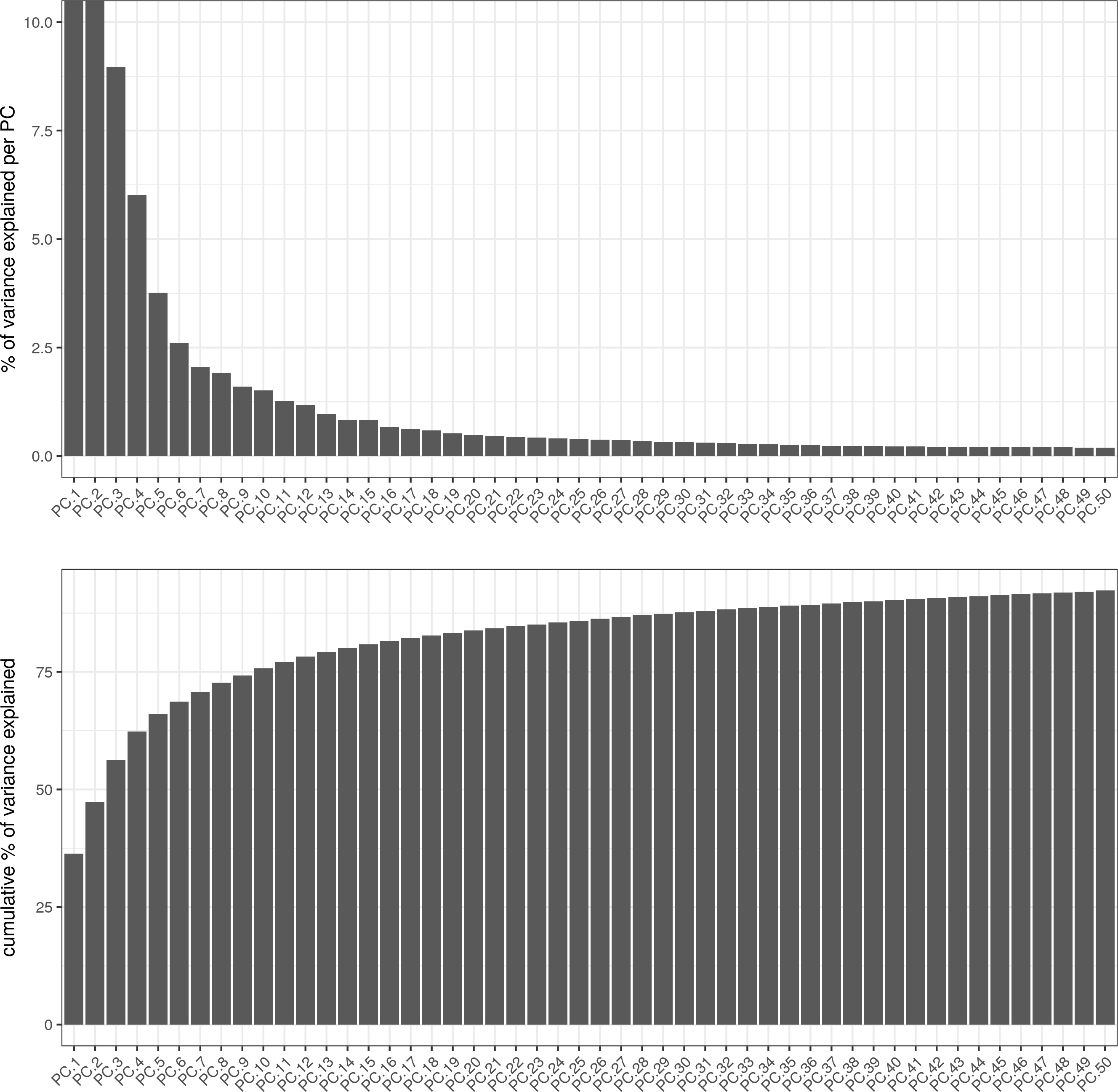
# significant PCs
signPCA(visium_brain, genes_to_use = featgenes, scale_unit = F)
plotPCA(gobject = visium_brain)

UMAP and tSNE

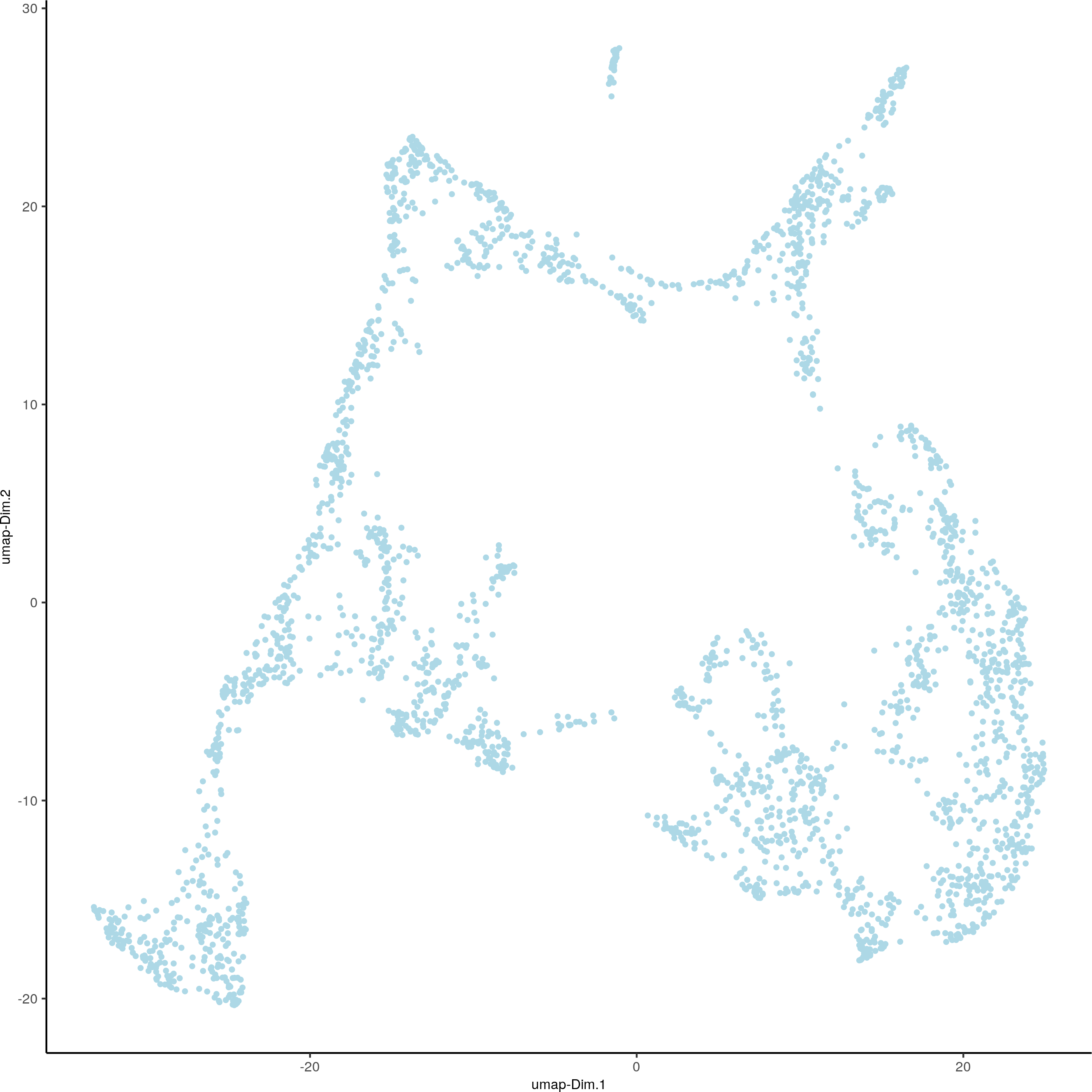
visium_brain <- runUMAP(visium_brain, dimensions_to_use = 1:10)
plotUMAP(gobject = visium_brain)
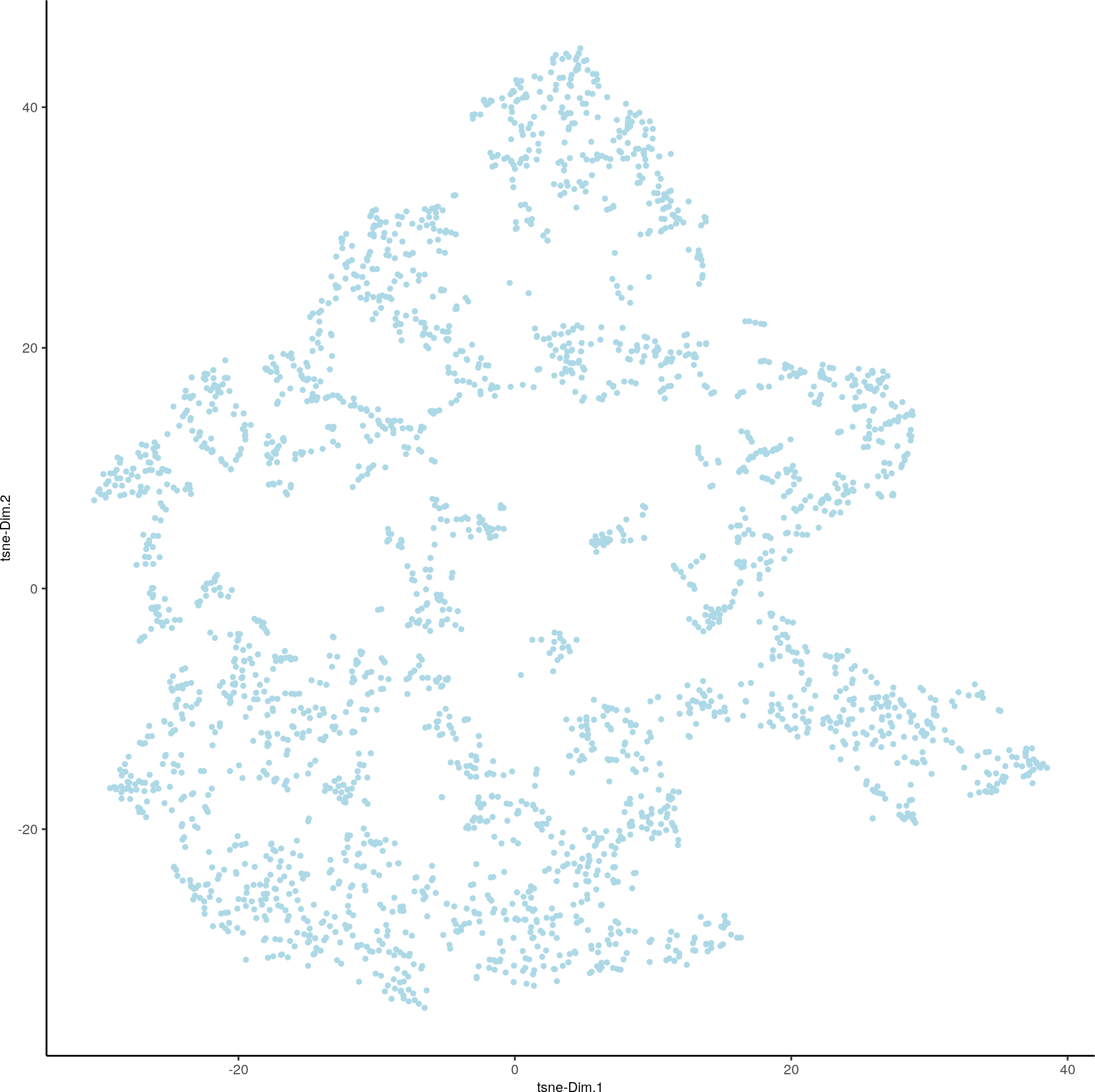
visium_brain <- runtSNE(visium_brain, dimensions_to_use = 1:10)
plotTSNE(gobject = visium_brain)

4. Clustering

We adopt a shared nearest neighbor approach. First create nearest network.

## sNN network (default)
visium_brain <- createNearestNetwork(gobject = visium_brain, dimensions_to_use = 1:10, k = 15)

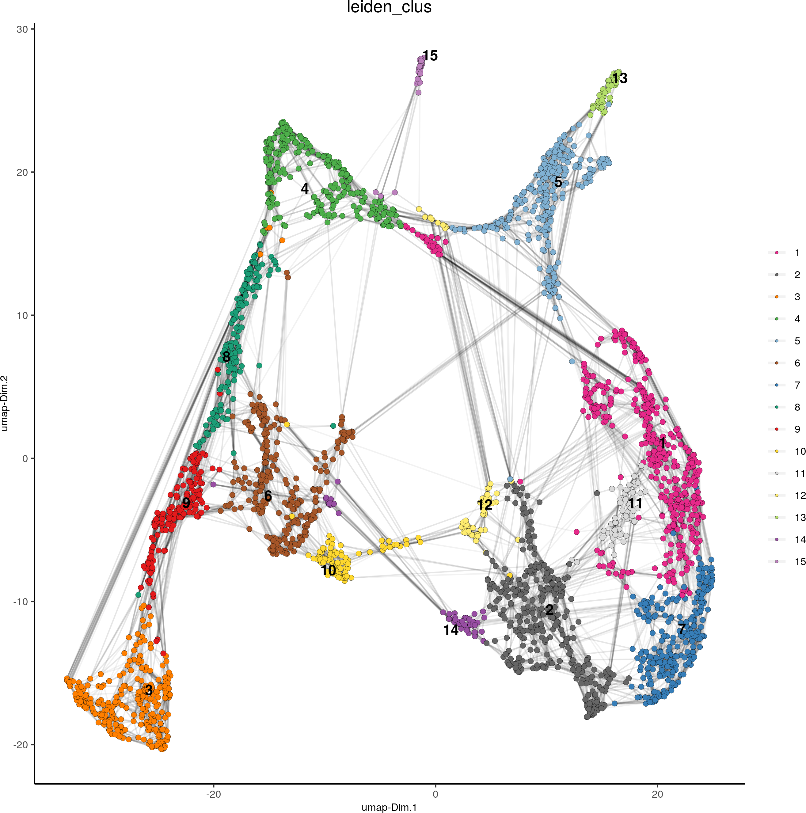
Leiden clustering

visium_brain <- doLeidenCluster(gobject = visium_brain, resolution = 0.4, n_iterations = 1000)
# default cluster result name from doLeidenCluster = 'leiden_clus'
plotUMAP(gobject = visium_brain, cell_color = 'leiden_clus', show_NN_network = T, point_size = 2)
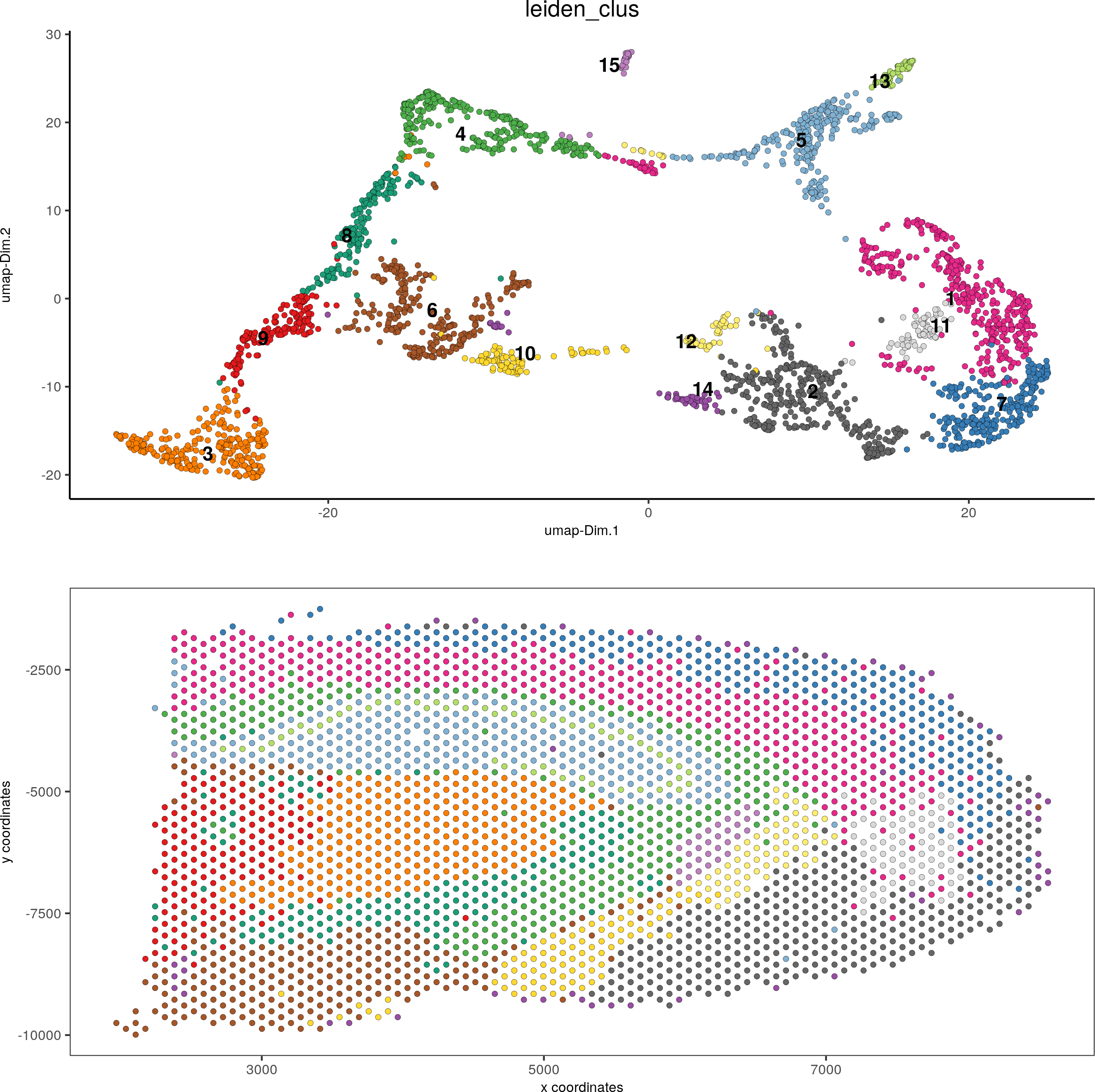
spatDimPlot(gobject = visium_brain, cell_color = 'leiden_clus',dim_point_size = 1.5, spat_point_size = 1.5)
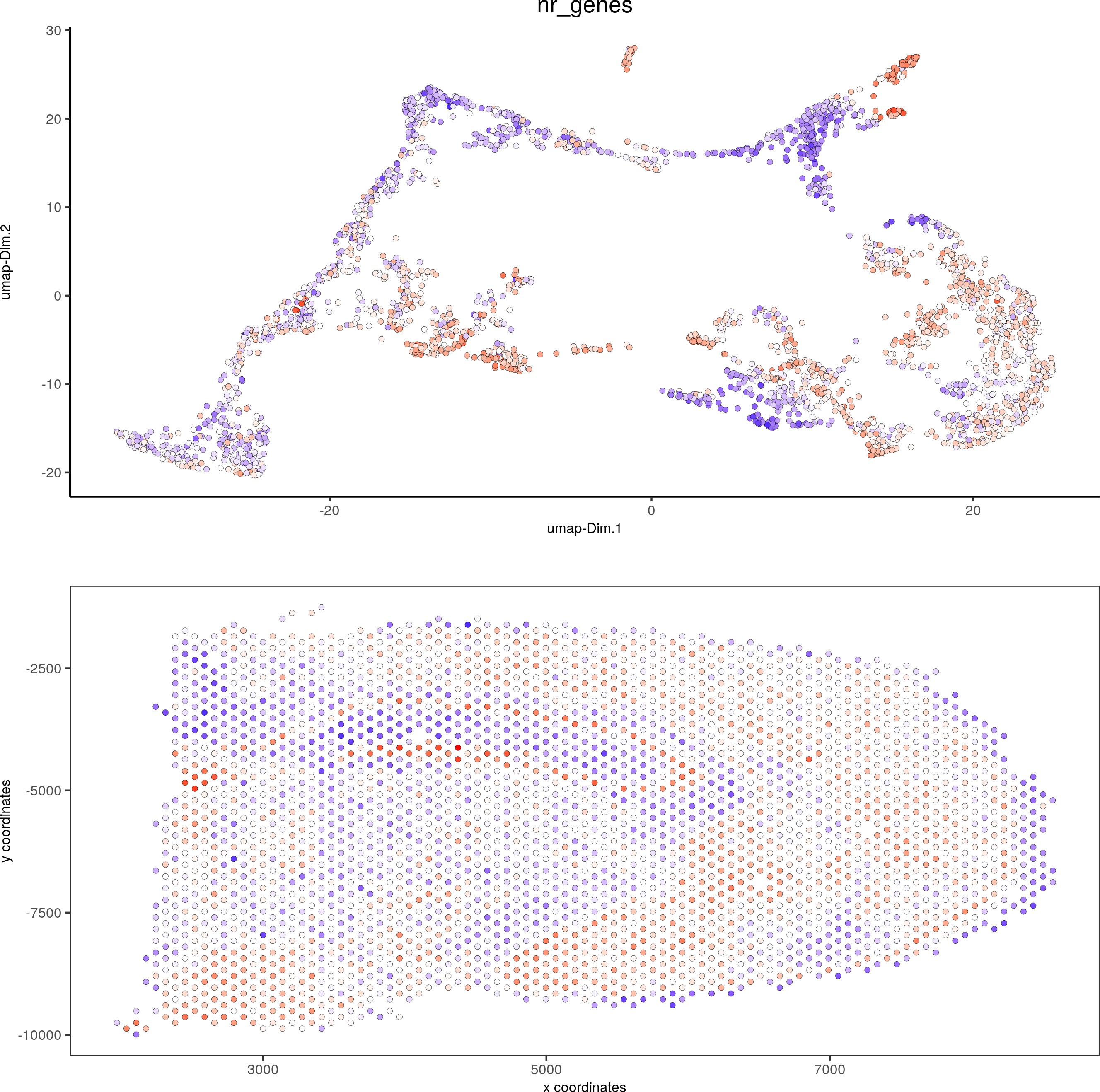
spatDimPlot(gobject = visium_brain, cell_color = 'nr_genes', color_as_factor = F,dim_point_size = 1.5, spat_point_size = 1.5)
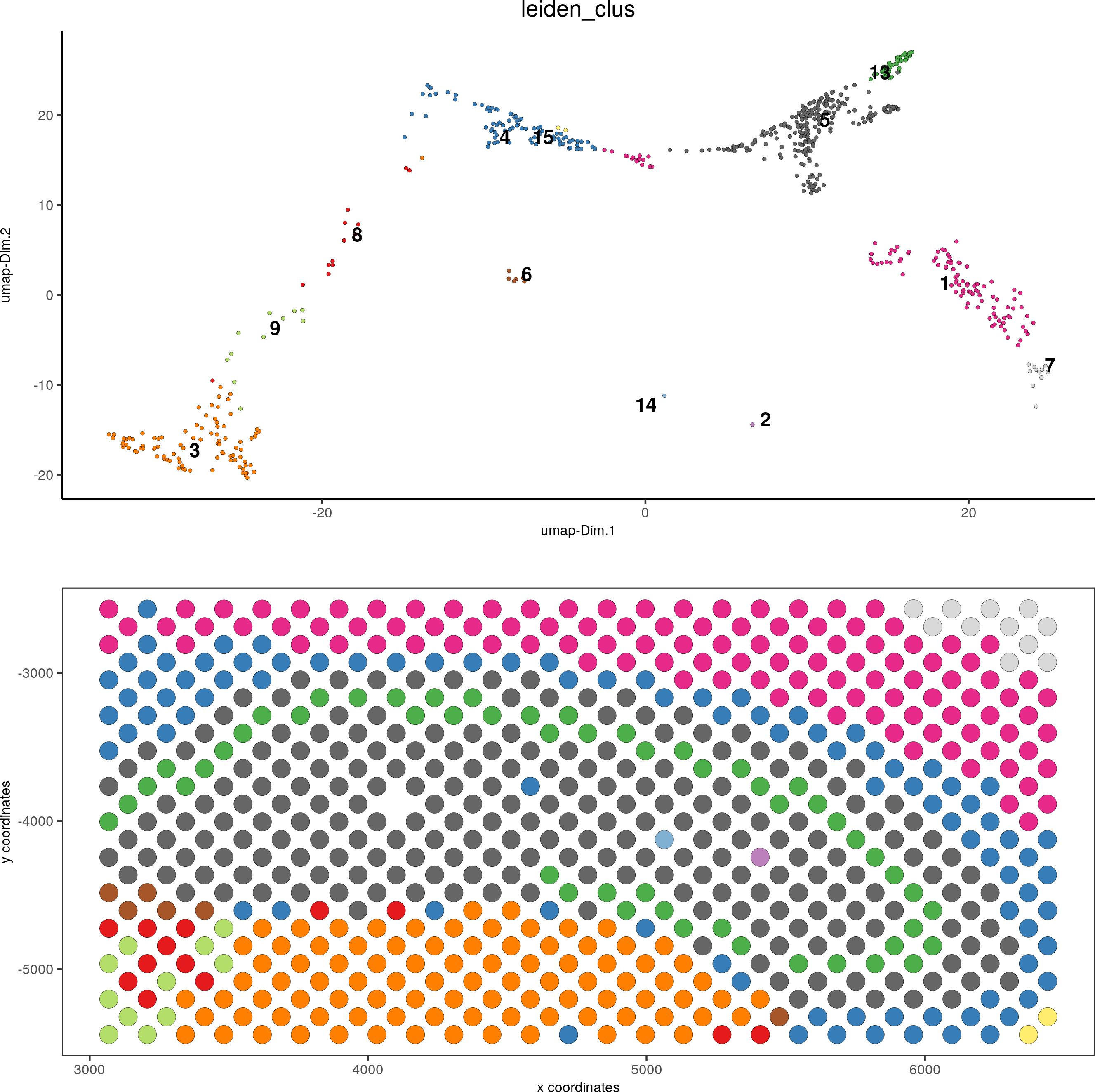
DG_subset = subsetGiottoLocs(visium_brain, x_max = 6500, x_min = 3000, y_max = -2500, y_min = -5500, return_gobject = T)
spatDimPlot(gobject = DG_subset, cell_color = 'leiden_clus', spat_point_size = 5)

5. Marker gene identification

We illustrate the Gini approach and the Scran approach.

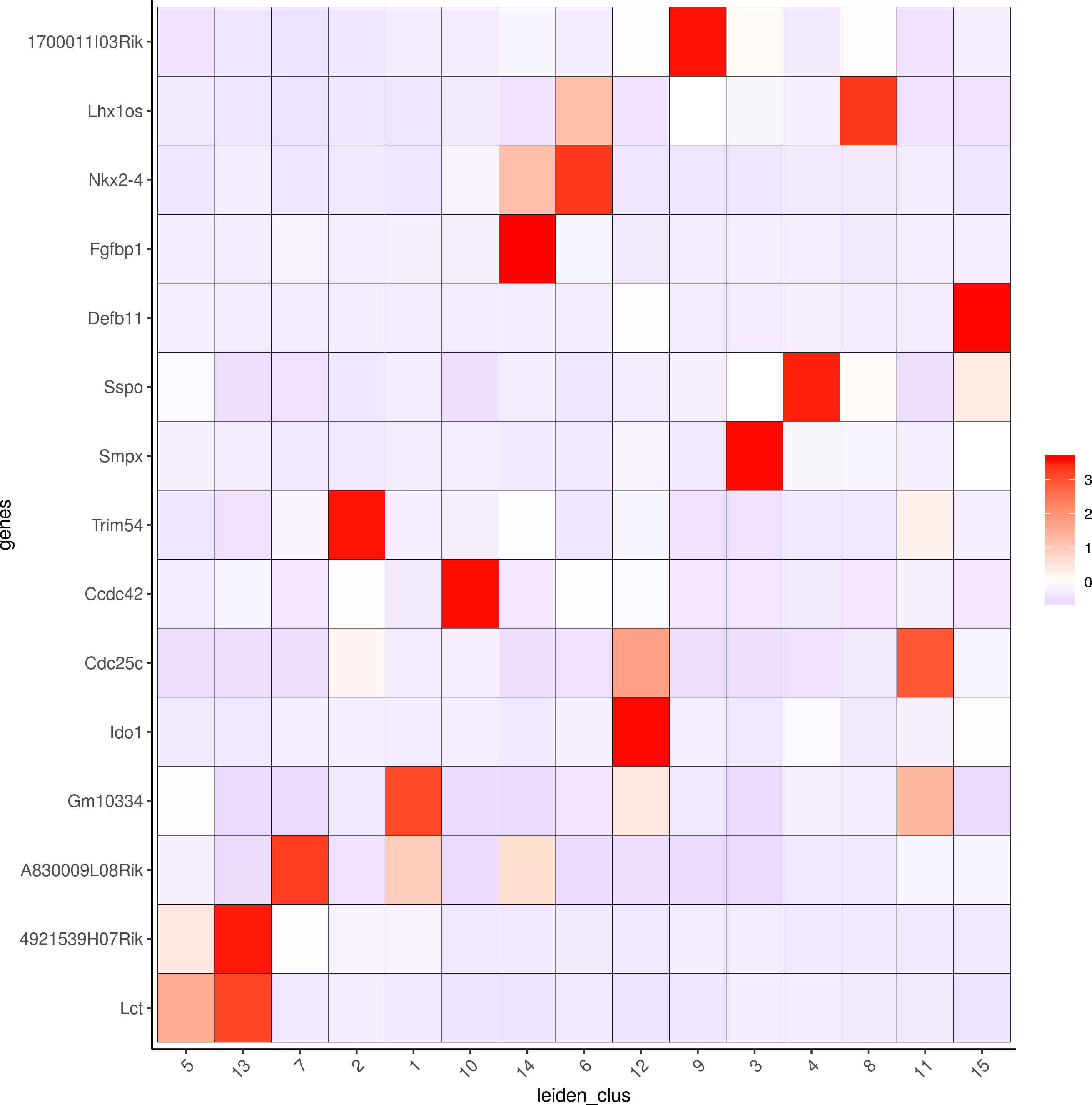
Gini

gini_markers_subclusters = findMarkers_one_vs_all(gobject = visium_brain,method = 'gini',expression_values = 'normalized',cluster_column = 'leiden_clus',min_genes = 20,min_expr_gini_score = 0.5,min_det_gini_score = 0.5)
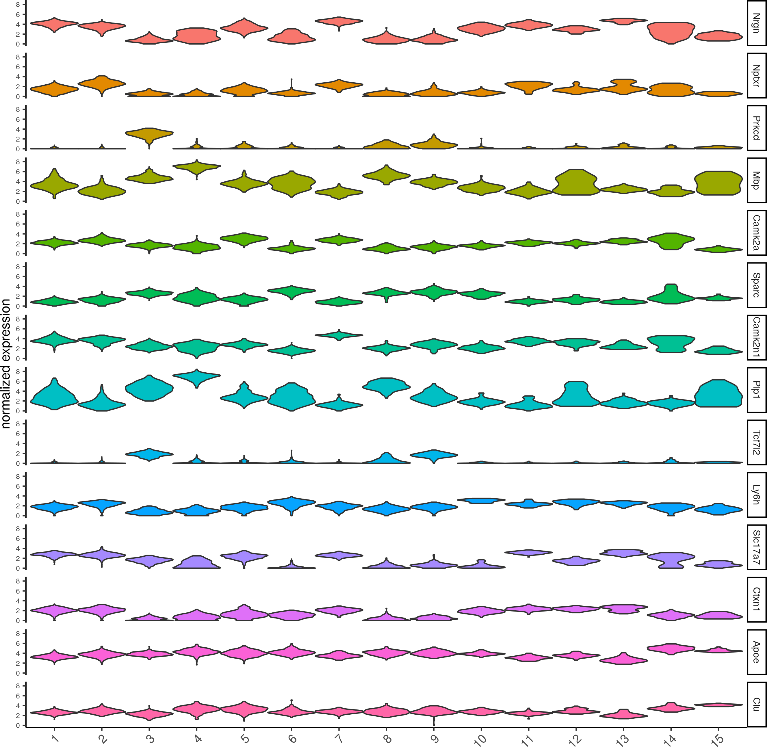
# violinplot
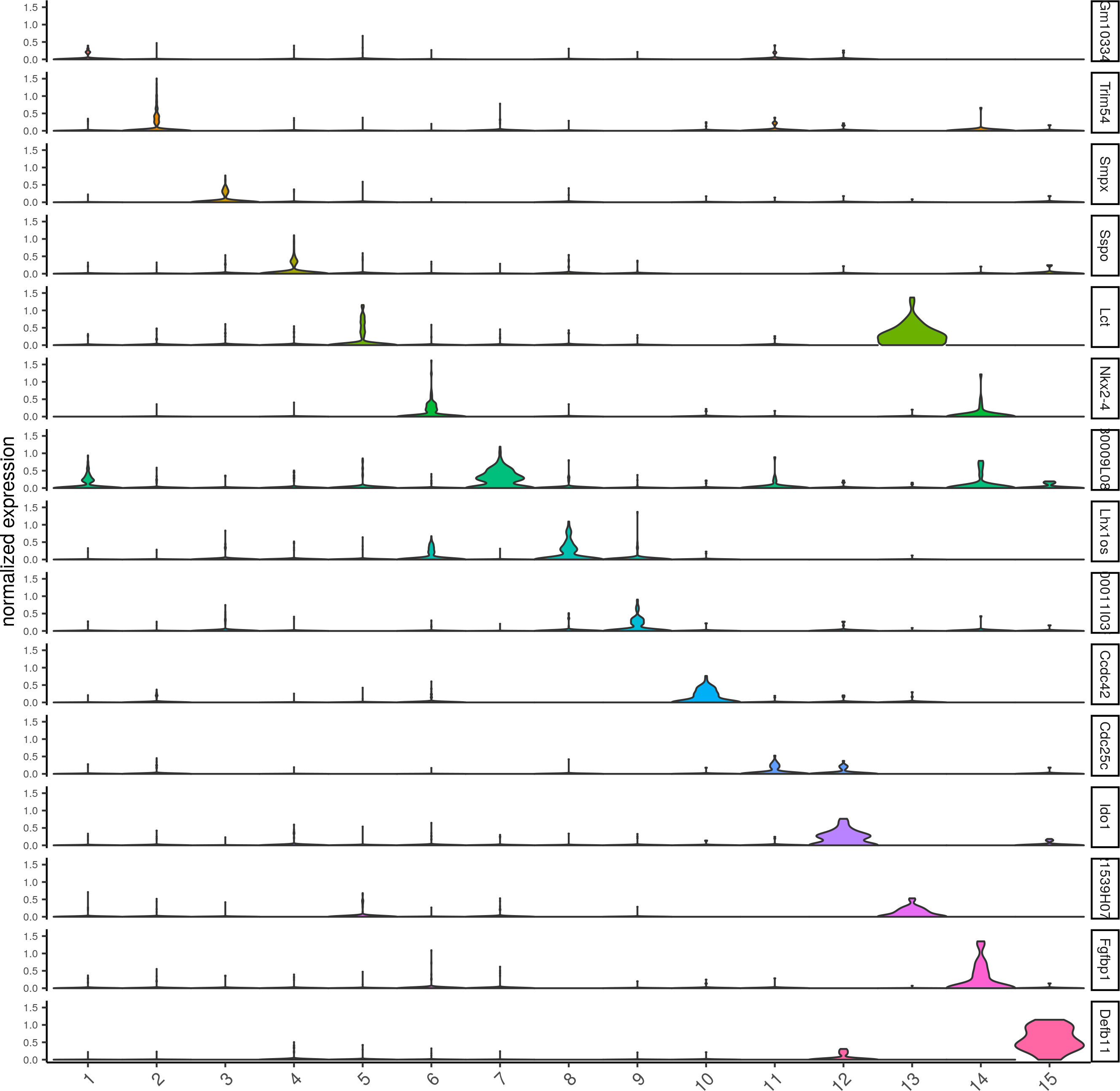
topgenes_gini = gini_markers_subclusters[, head(.SD, 1), by = 'cluster']$genes
violinPlot(visium_brain, genes = unique(topgenes_gini), cluster_column = 'leiden_clus',strip_text = 8, strip_position = 'right')

topgenes_gini = gini_markers_subclusters[, head(.SD, 2), by = 'cluster']$genes
my_cluster_order = c(5, 13, 7, 2, 1, 10, 14, 6, 12, 9, 3, 4 , 8, 11, 15)
plotMetaDataHeatmap(visium_brain, selected_genes = topgenes_gini, custom_cluster_order = my_cluster_order, metadata_cols = c('leiden_clus'), x_text_size = 10, y_text_size = 10)

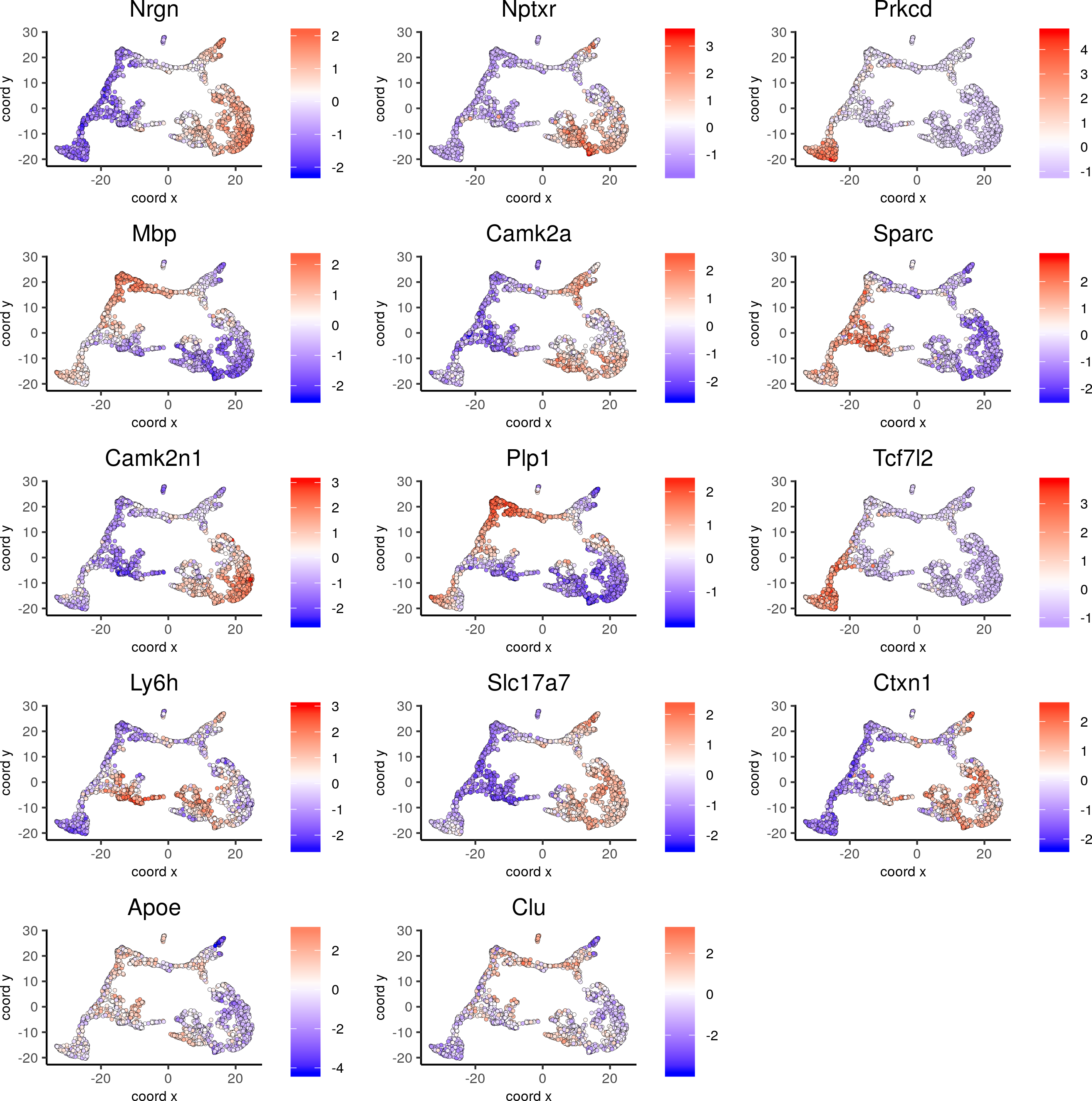
dimGenePlot2D(visium_brain, expression_values = 'scaled',genes = gini_markers_subclusters[, head(.SD, 1), by = 'cluster']$genes,cow_n_col = 3, point_size = 1)

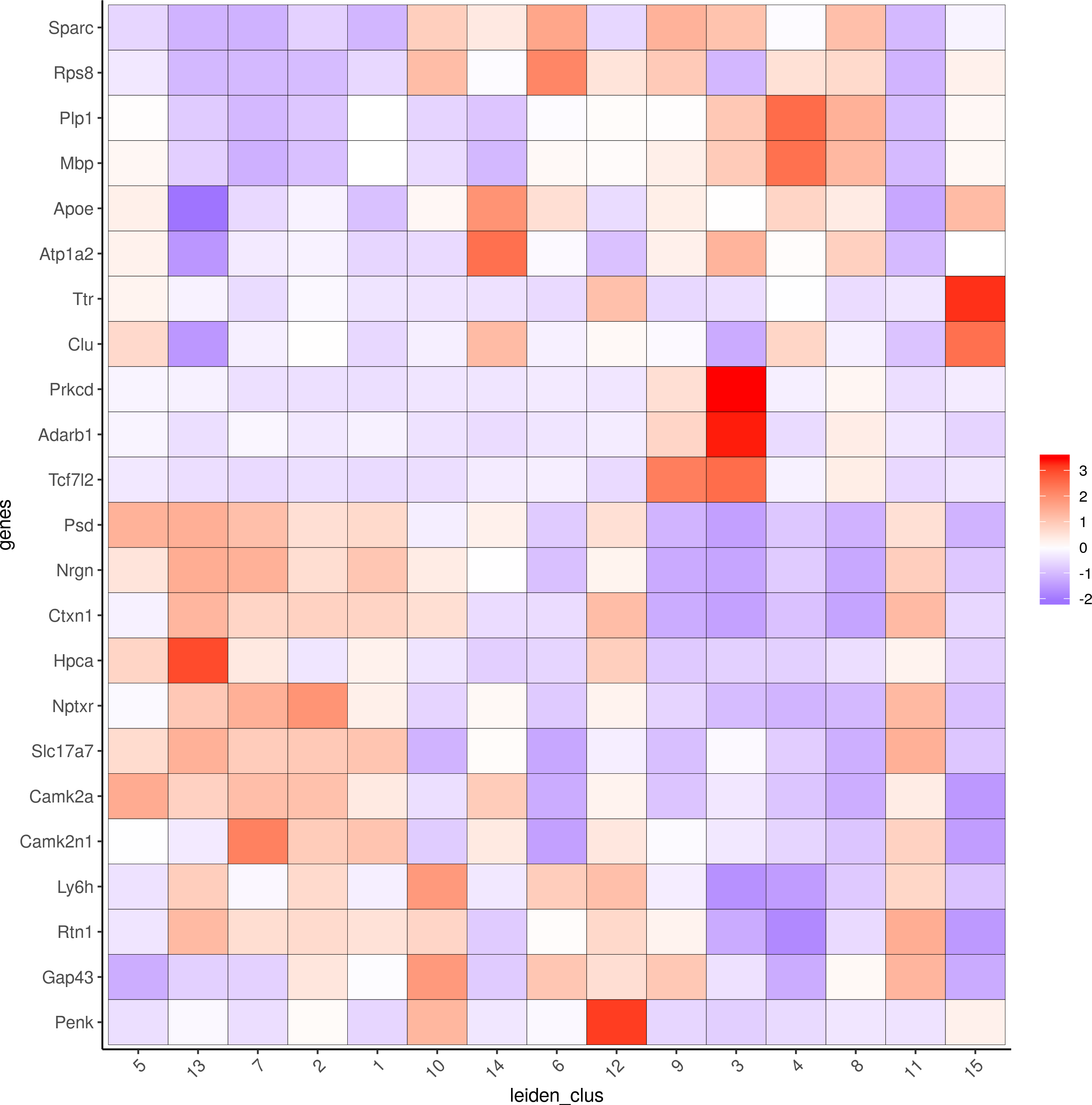
Scran

scran_markers_subclusters = findMarkers_one_vs_all(gobject = visium_brain,method = 'scran',expression_values = 'normalized',cluster_column = 'leiden_clus')
# violinplot
topgenes_scran = scran_markers_subclusters[, head(.SD, 1), by = 'cluster']$genes
violinPlot(visium_brain, genes = unique(topgenes_scran), cluster_column = 'leiden_clus',strip_text = 8, strip_position = 'right')

topgenes_scran = scran_markers_subclusters[, head(.SD, 2), by = 'cluster']$genes
plotMetaDataHeatmap(visium_brain, selected_genes = topgenes_scran, custom_cluster_order = my_cluster_order,metadata_cols = c('leiden_clus'))
# umap plots
dimGenePlot2D(visium_brain, expression_values = 'scaled',genes = scran_markers_subclusters[, head(.SD, 1), by = 'cluster']$genes,cow_n_col = 3, point_size = 1)

6. Cell type enrichment.

Visium spatial transcriptomics does not provide single-cell resolution, making cell type annotation a harder problem. Giotto provides 3 ways to calculate enrichment of specific cell-type signature gene list:

• PAGE
• rank
• hypergeometric test

To generate the cell-type specific gene lists for the mouse brain data we used cell-type specific gene sets as identified in Zeisel, A. et al. Molecular Architecture of the Mouse Nervous System. Here we illustrate the PAGE enrichment method.

Load cell type signature genes

Signature matrix is a binary (0/1) matrix. Rows are genes. Columns are cell types.

# known markers for different mouse brain cell types:
# Zeisel, A. et al. Molecular Architecture of the Mouse Nervous System. Cell 174, 999-1014.e22 (2018).
## cell type signatures ##
## combination of all marker genes identified in Zeisel et al
brain_sc_markers = data.table::fread(fs::path(workdir, 'sig_matrix.txt')) # file don't exist in data folder
sig_matrix = as.matrix(brain_sc_markers[,-1]); rownames(sig_matrix) = brain_sc_markers$Event

Run PAGE enrichment test

visium_brain = createSpatialEnrich(visium_brain, sign_matrix = sig_matrix, enrich_method = 'PAGE') #default = 'PAGE'

Visualize the results

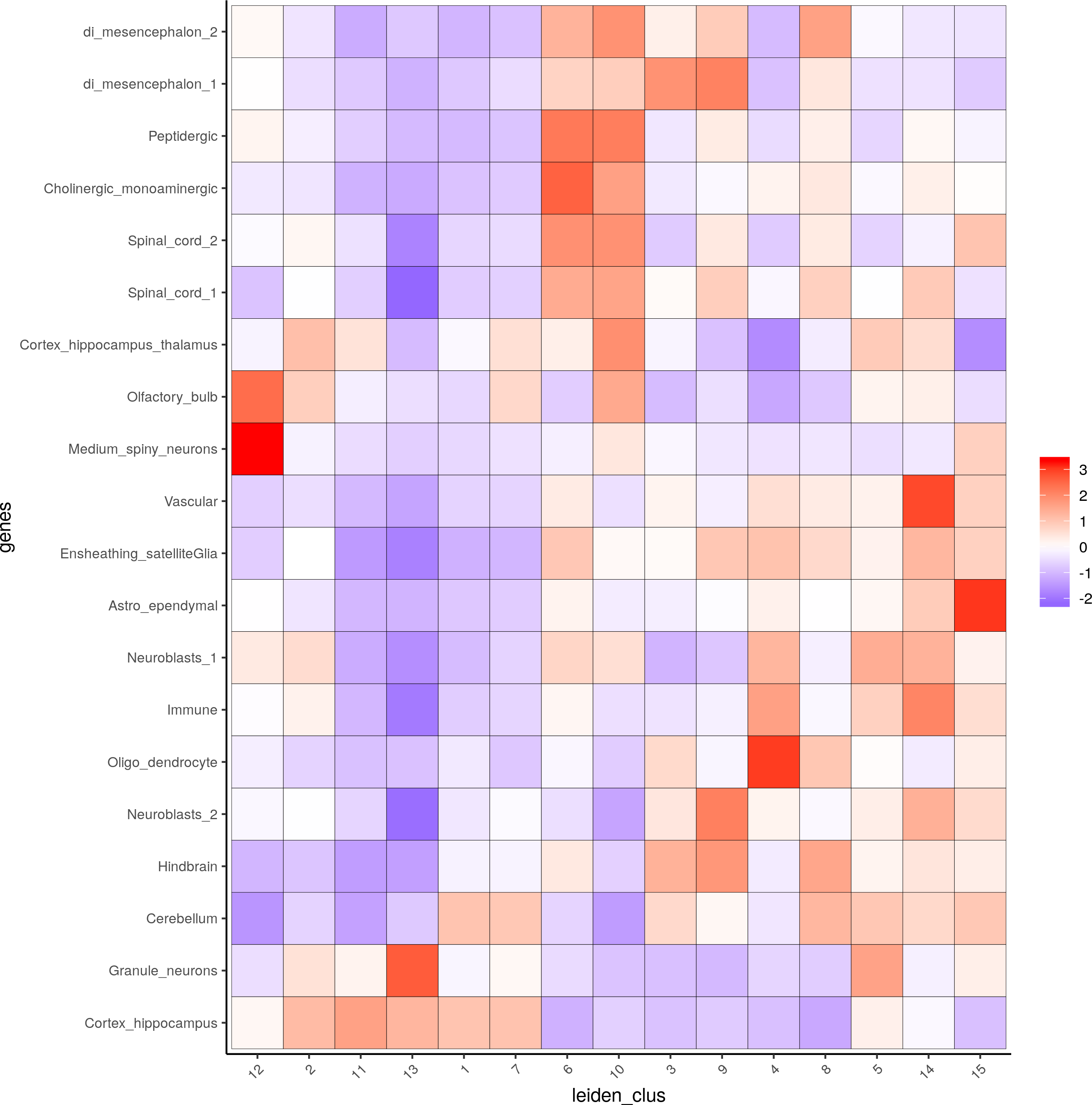
## heatmap of enrichment versus annotation (e.g. clustering result)
cell_types = colnames(sig_matrix)
plotMetaDataCellsHeatmap(gobject = visium_brain,metadata_cols = 'leiden_clus',value_cols = cell_types,spat_enr_names = 'PAGE',x_text_size = 8, y_text_size = 8)

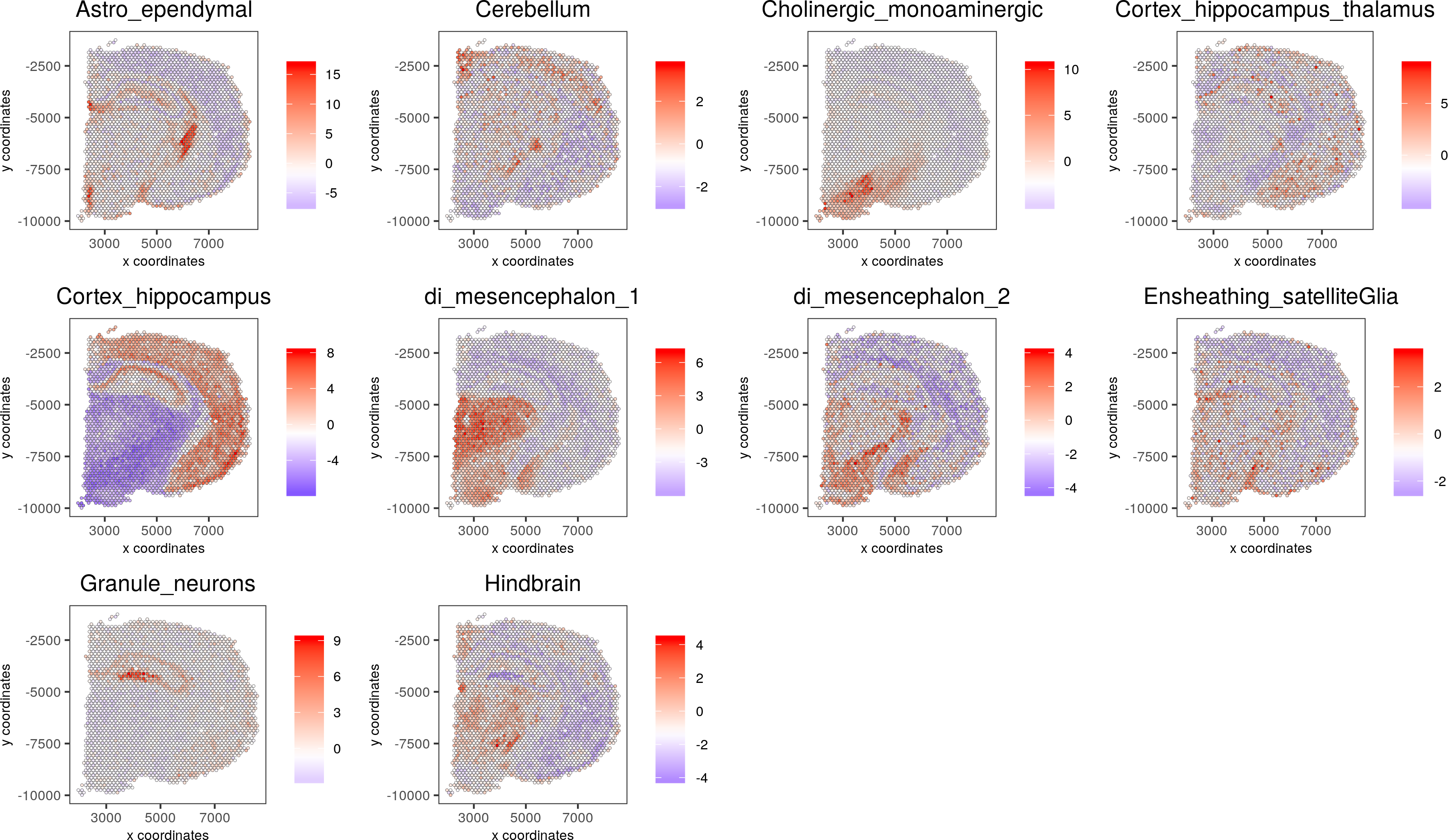
Visualize the key cell type enrichment results

cell_types_subset = colnames(sig_matrix)[1:10]
spatCellPlot(gobject = visium_brain, spat_enr_names = 'PAGE',cell_annotation_values = cell_types_subset,cow_n_col = 4,coord_fix_ratio = NULL, point_size = 0.75)
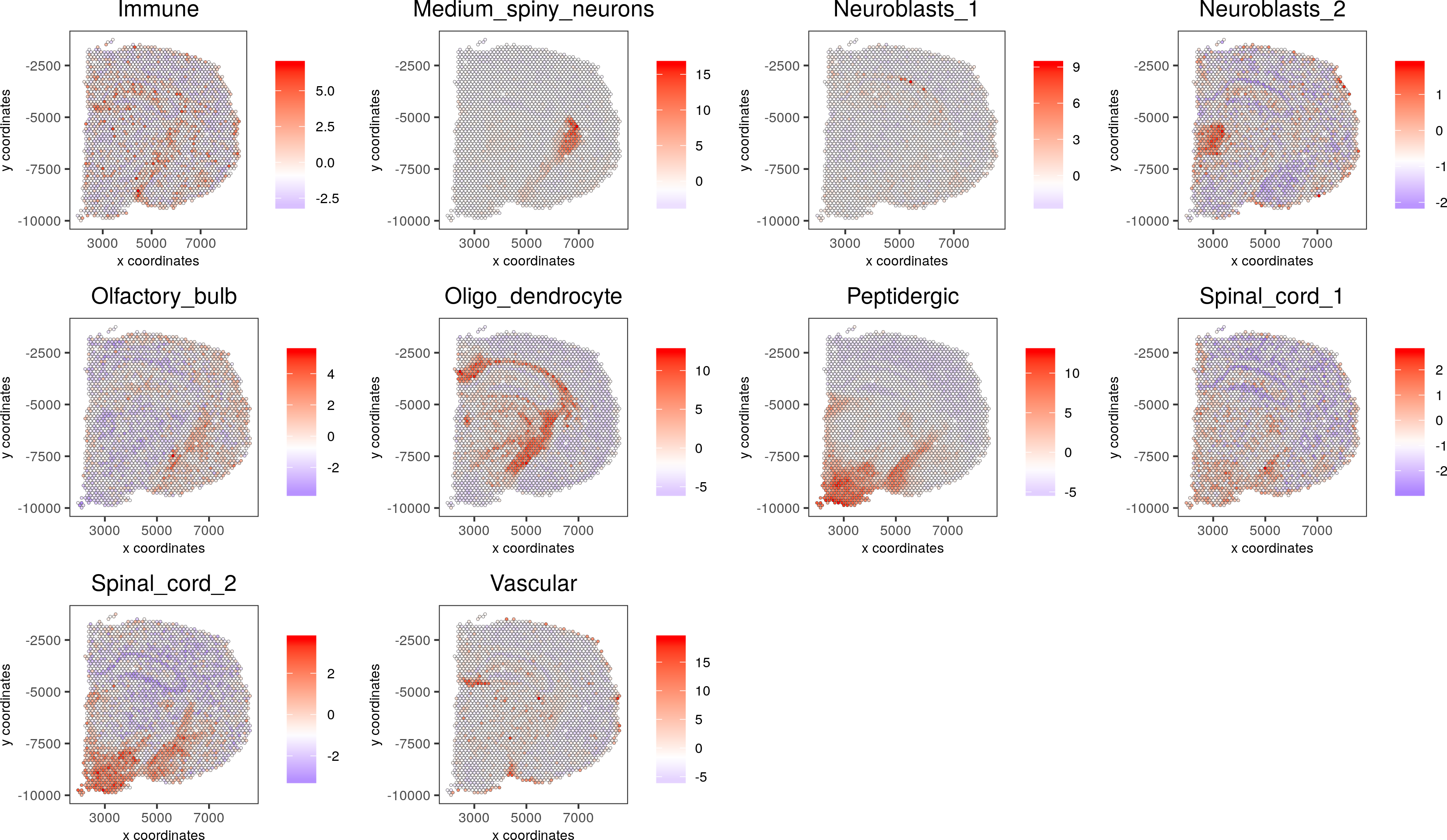
cell_types_subset = colnames(sig_matrix)[11:20]
spatCellPlot(gobject = visium_brain, spat_enr_names = 'PAGE', cell_annotation_values = cell_types_subset, cow_n_col = 4,coord_fix_ratio = NULL, point_size = 0.75)

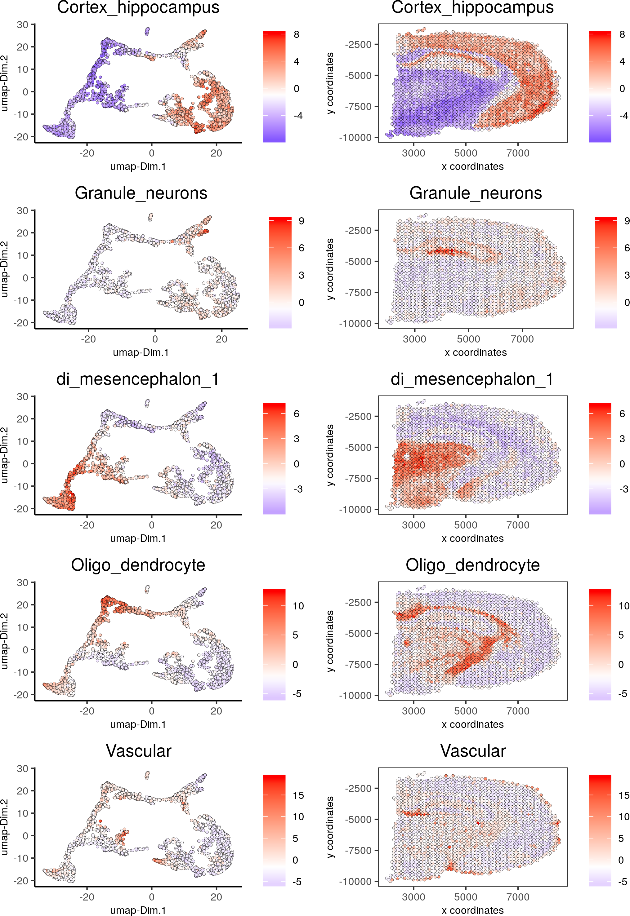
spatDimCellPlot(gobject = visium_brain, spat_enr_names = 'PAGE',cell_annotation_values = c('Cortex_hippocampus', 'Granule_neurons', 'di_mesencephalon_1', 'Oligo_dendrocyte','Vascular'),cow_n_col = 1, spat_point_size = 1, plot_alignment = 'horizontal')

7. Spatial gene detection

We illustrate 3 ways of finding spatial genes, though Giotto also supports a number of other ways that we did not develop but which we created wrappers. We illustrate binSpect (kmeans), binSpect (rank), and silhouetteRank.

We first create a spatial network which is needed for binSpect, and for later HMRF based analysis.

Spatial network

# create spatial grid
visium_brain <- createSpatialGrid(gobject = visium_brain, sdimx_stepsize = 400, sdimy_stepsize = 400, minimum_padding = 0)
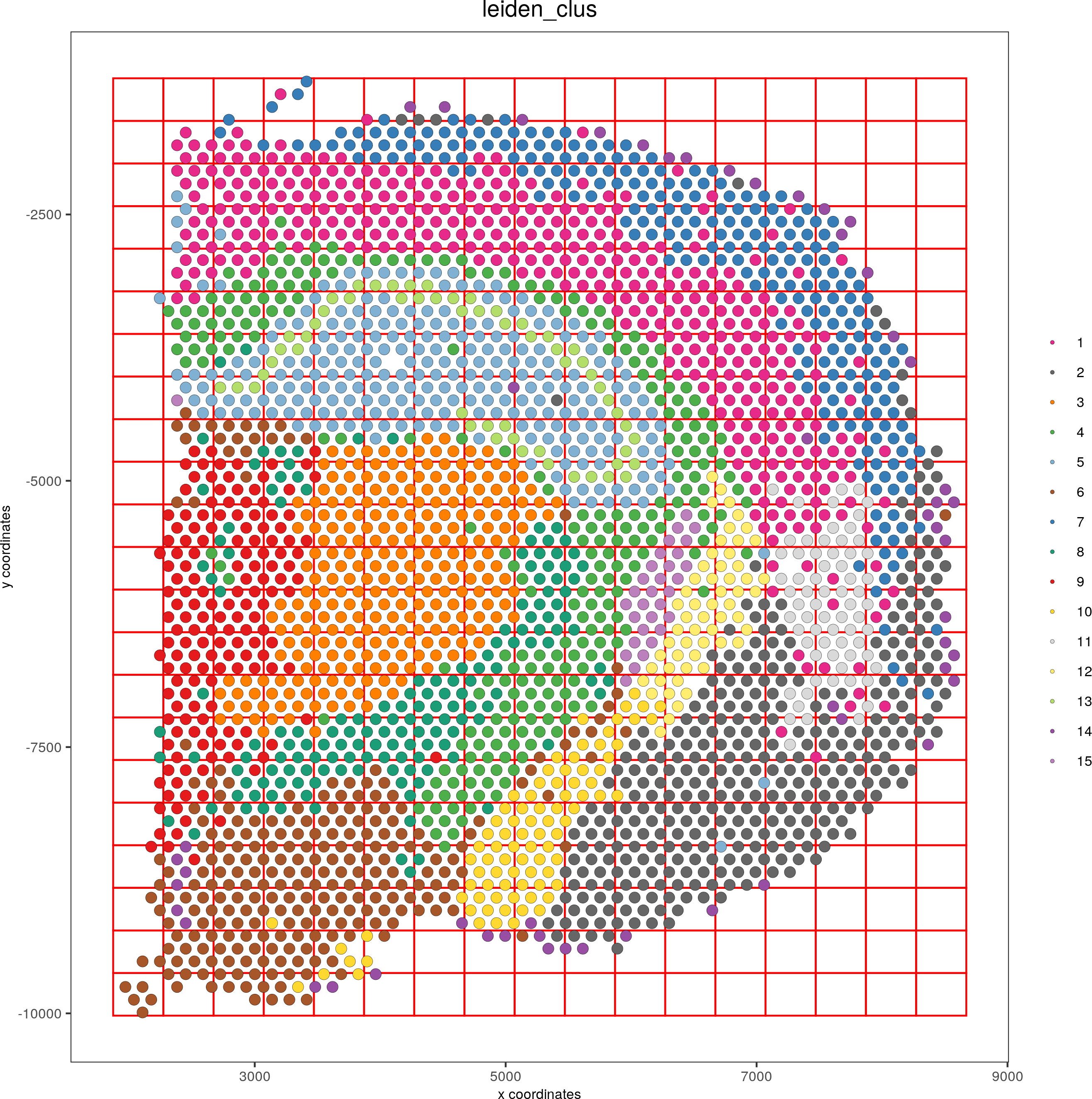
spatPlot(visium_brain, cell_color = 'leiden_clus', show_grid = T, grid_color = 'red', spatial_grid_name = 'spatial_grid')
# create spatial network
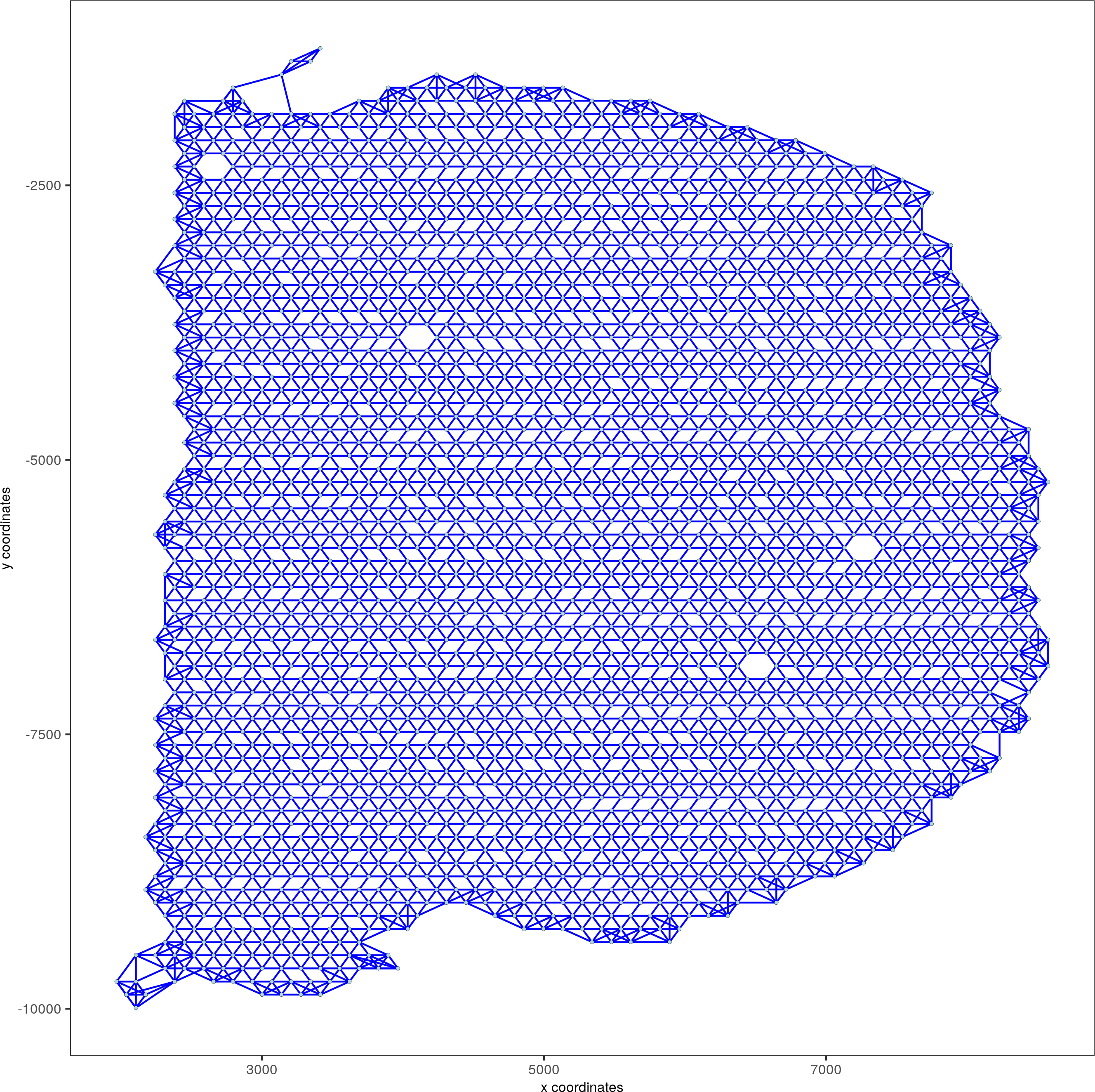
visium_brain <- createSpatialNetwork(gobject = visium_brain, method = 'kNN', k = 5, maximum_distance_knn = 400, name = 'spatial_network')
spatPlot(gobject = visium_brain, show_network = T, point_size = 1, network_color = 'blue', spatial_network_name = 'spatial_network')

Spatial gene method

Then we call binSpect (kmeans) and binSpect (rank), and silhouetteRank. In reality, calling just one of these spatial gene methods is enough.

Sys.time()
kmtest = binSpect(visium_brain, calc_hub = T, hub_min_int = 5,spatial_network_name = 'spatial_network')
spatGenePlot(visium_brain, expression_values = 'scaled',genes = kmtest$genes[1:6], cow_n_col = 2, point_size = 1)
Sys.time()
## rank binarization
ranktest = binSpect(visium_brain, bin_method = 'rank', calc_hub = T, hub_min_int = 5,spatial_network_name = 'spatial_network')
spatGenePlot(visium_brain, expression_values = 'scaled',genes = ranktest$genes[1:6], cow_n_col = 2, point_size = 1)
Sys.time()
## silhouette
spatial_genes=silhouetteRankTest(visium_brain, overwrite_input_bin=F, output="sil.result", matrix_type="dissim", num_core=4, parallel_path="/usr/bin", verbose=T, expression_values="norm", query_sizes=10)

Visualize the results of silhouetteRank:

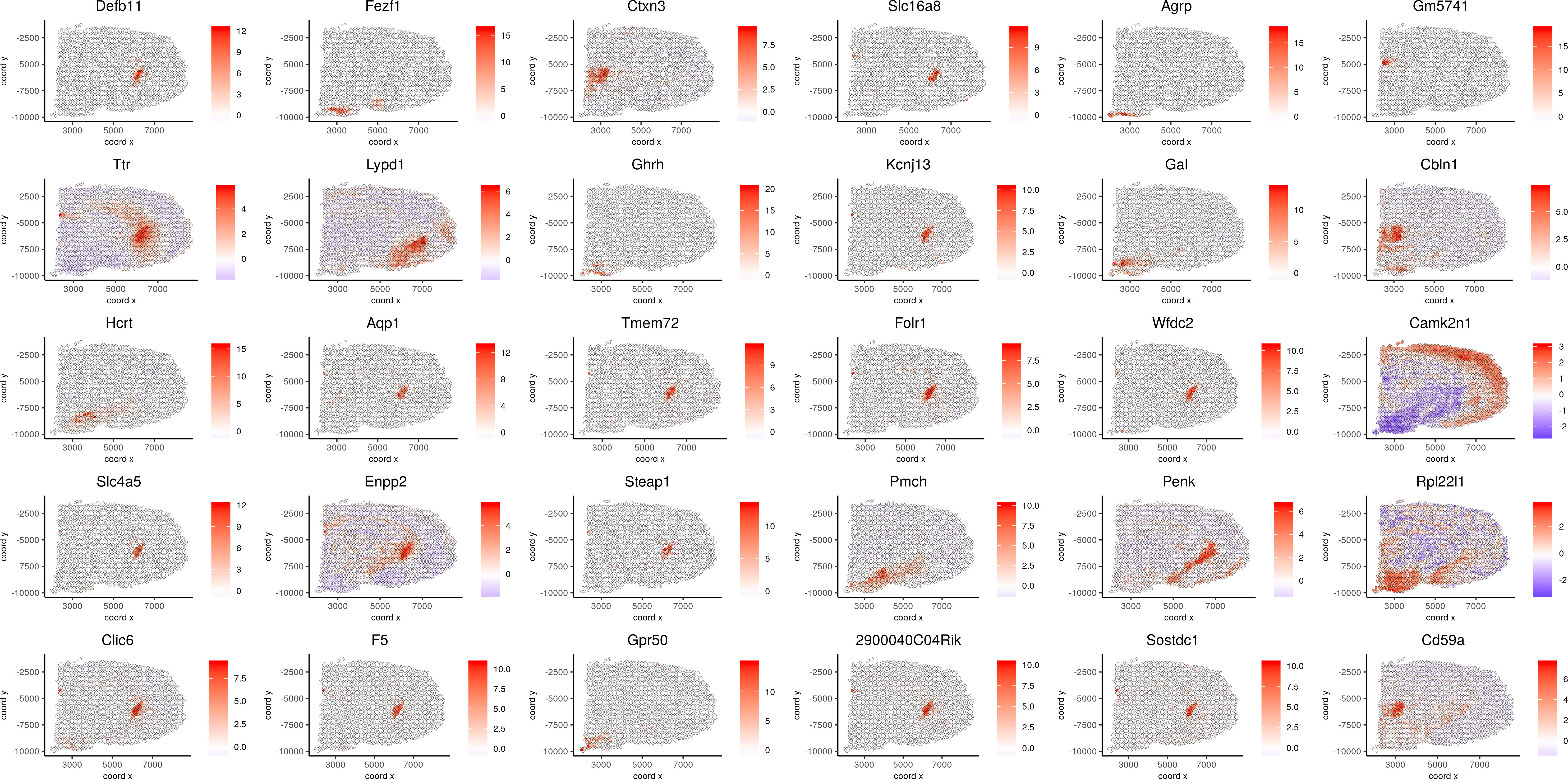
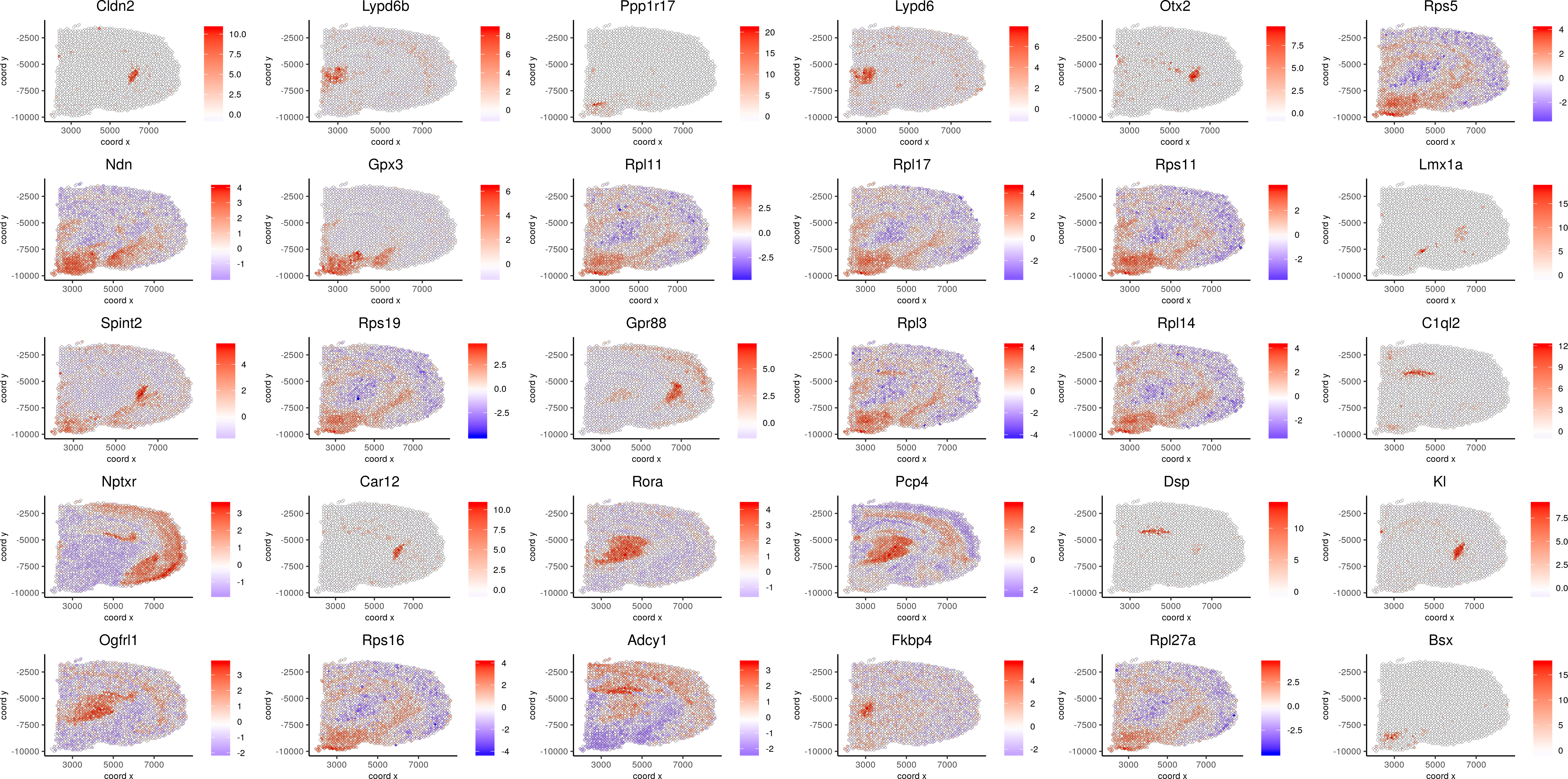
spatGenePlot(visium_brain, expression_values = 'scaled',genes = spatial_genes$gene[1:30], cow_n_col = 6, point_size = 1, save_param=c(base_width=20, base_height=10))
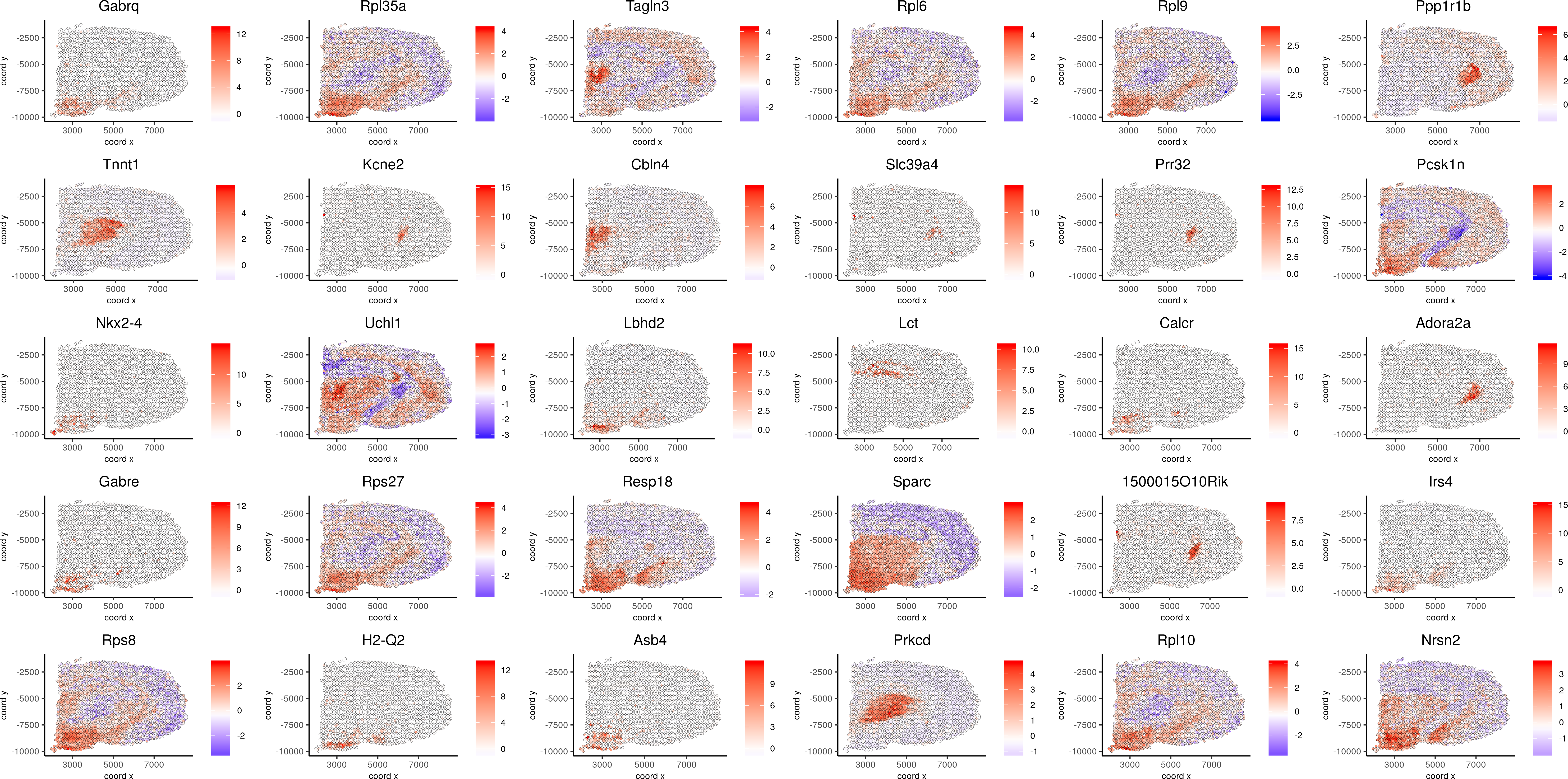
spatGenePlot(visium_brain, expression_values = 'scaled',genes = spatial_genes$gene[31:60], cow_n_col = 6, point_size = 1, save_param=c(base_width=20, base_height=10))
spatGenePlot(visium_brain, expression_values = 'scaled',genes = spatial_genes$gene[61:90], cow_n_col = 6, point_size = 1, save_param=c(base_width=20, base_height=10))

Spatial Genes 1-30:

Spatial Genes 31-60:

Spatial Genes 61-90:

8. Spatial domains detection by HMRF

We begin with spatial genes detected in the previous step. Rank genes by spatial scores (silhouetteRank)

plot(x=seq(1, 14414), y=-log10(spatial_genes$pval), xlab="Rank of genes by spatial score", ylab="-log10Pvalue")
abline(v=c(1500))

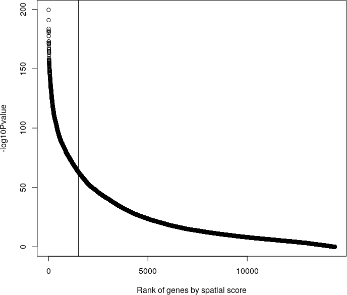
Cluster the top 1500 spatial genes into 20 clusters

ext_spatial_genes = spatial_genes[1:1500,]$gene

Here we use existing detectSpatialCorGenes function to calculate pairwise distances between genes (but set network_smoothing=0 to use default clustering without smoothing)

spat_cor_netw_DT = detectSpatialCorGenes(visium_brain, method = 'network', spatial_network_name = 'spatial_network', subset_genes = ext_spatial_genes, network_smoothing=0)
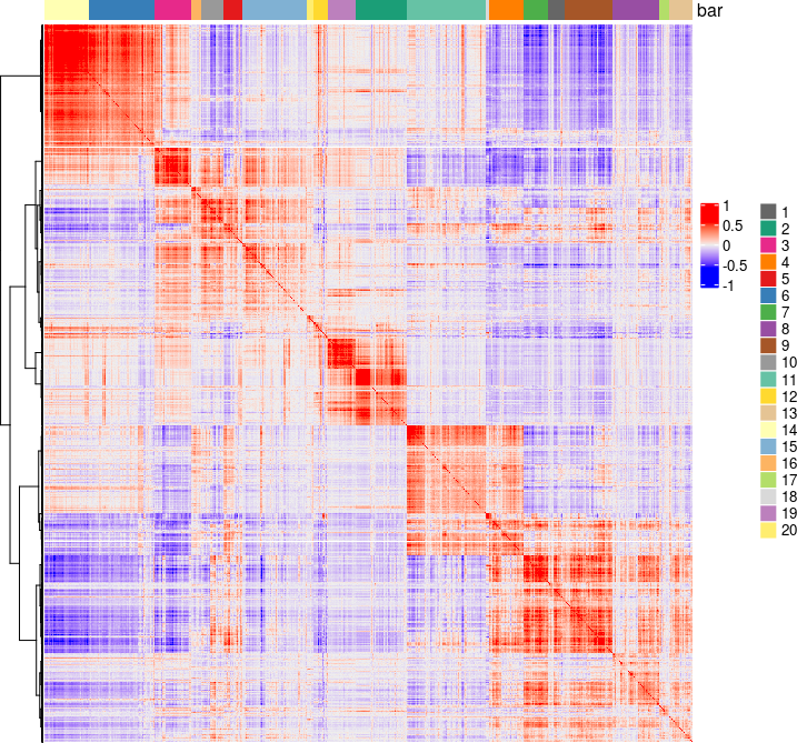
# cluster spatial genes
spat_cor_netw_DT = clusterSpatialCorGenes(spat_cor_netw_DT, name = 'spat_netw_clus', k = 20)
# visualize clusters
heatmSpatialCorGenes(visium_brain, spatCorObject = spat_cor_netw_DT, use_clus_name = 'spat_netw_clus', heatmap_legend_param = list(title = NULL))

Sample the spatial genes at a per cluster basis, but different from regular sampling, sampling is based on cluster size, controlled by sample_rate (between 1 to 10. 1 means equal number per cluster, 10 means number of samples is directly proportional to cluster size) Target number of spatial genes = 500

sample_rate=2
target=500
tot=0
num_cluster=20
gene_list = list()
clust = spat_cor_netw_DT$cor_clusters$spat_netw_clus
for(i in seq(1, num_cluster)){
    gene_list[[i]] = colnames(t(clust[which(clust==i)]))
}
for(i in seq(1, num_cluster)){
    num_g=length(gene_list[[i]])
    tot = tot+num_g/(num_g^(1/sample_rate))
}
factor=target/tot
num_sample=c()
for(i in seq(1, num_cluster)){
    num_g=length(gene_list[[i]])
    num_sample[i] = round(num_g/(num_g^(1/sample_rate)) * factor)
}
set.seed(10)
samples=list()
union_genes = c()
for(i in seq(1, num_cluster)){
    if(length(gene_list[[i]])<num_sample[i]){
        samples[[i]] = gene_list[[i]]
    }else{
        samples[[i]] = sample(gene_list[[i]], num_sample[i])
    }
    union_genes = union(union_genes, samples[[i]])
}
union_genes = unique(union_genes)

Run HMRF routine

# do HMRF with different betas on 500 spatial genes
my_spatial_genes <- union_genes
hmrf_folder = fs::path("11_HMRF")
if(!file.exists(hmrf_folder)) dir.create(hmrf_folder, recursive = T)
HMRF_spatial_genes = doHMRF(gobject = visium_brain, expression_values = 'scaled', spatial_genes = my_spatial_genes, k = 20,   spatial_network_name="spatial_network", betas = c(0, 10, 5),  output_folder = paste0(hmrf_folder, '/', 'Spatial_genes/SG_topgenes_k20_scaled'))

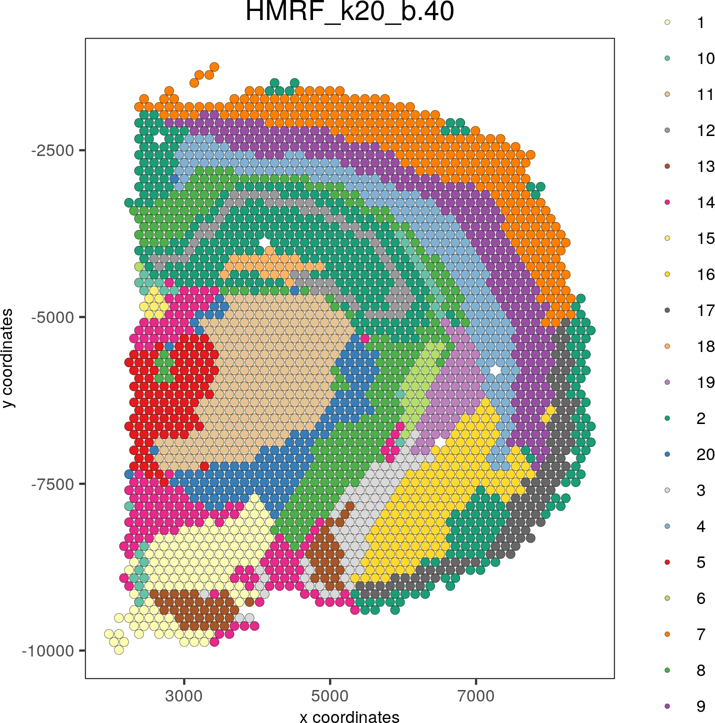
Visualize HMRF result

visium_brain = addHMRF(gobject = visium_brain, HMRFoutput = HMRF_spatial_genes, k = 20, betas_to_add = c(0, 10, 20, 30, 40), hmrf_name = 'HMRF')
spatPlot(gobject = visium_brain, cell_color = 'HMRF_k20_b.40', point_size = 2)

Part 9. Export Giotto data to viewer

# check which annotations are available
combineMetadata(visium_brain, spat_enr_names = 'PAGE')
# select annotations, reductions and expression values to view in Giotto Viewer
results_folder=workdir
viewer_folder = fs::path(results_folder, "mouse_visium_brain_viewer")
exportGiottoViewer(gobject = visium_brain, output_directory = viewer_folder, spat_enr_names = 'PAGE', factor_annotations = c('in_tissue','leiden_clus','HMRF_k20_b.30'), numeric_annotations = c('nr_genes', 'clus_25'), dim_reductions = c('tsne', 'umap'), dim_reduction_names = c('tsne', 'umap'), expression_values = 'scaled', expression_rounding = 2, overwrite_dir = T)

#================================================================ 
#Next steps. Please manually run the following in a SHELL terminal: 
#================================================================ 
cd  /data/mouse_visium_brain_viewer 
giotto_setup_image --require-stitch=n --image=n --image-multi-channel=n --segmentation=n --multi-fov=n --output-json=step1.json 
smfish_step1_setup -c step1.json 
giotto_setup_viewer --num-panel=2 --input-preprocess-json=step1.json --panel-1=PanelPhysicalSimple --panel-2=PanelTsne --output-json=step2.json --input-annotation-list=annotation_list.txt 
smfish_read_config -c step2.json -o test.dec6.js -p test.dec6.html -q test.dec6.css 
giotto_copy_js_css --output . 
python3 -m http.server 
================================================================ 
#Finally, open your browser, navigate to http://localhost:8000/. Then click on the file test.dec6.html to see the viewer.