merFISH dataset

0. Environment

library(Giotto)
# STOP!
# ====== 1. set working directory ======
# For Docker, set my_working_dir to /data
my_working_dir = '/data'
# For native install users, set my_working_dir to a directory accessible by user
#my_working_dir = "/home/qzhu/Downloads"
# ====== 2. set giotto python path ======
# For Docker, set python_path to /usr/bin/python3
python_path = "/usr/bin/python3"
# For native install users, python path may be different, and may depend on whether conda or virtual environment. One can check by "reticulate::py_discover_config()" to see which python is picked up automatically. Then set python_path to what is returned by py_discover_config.
# python_path = "/usr/bin/python3"

1. Preparation steps

1.1. Dataset explanation

Moffitt et al. created a 3D spatial expression dataset consisting of 155 genes from ~1 million single cells acquired over the mouse hypothalamic preoptic regions.

1.2 Dataset download

The merFISH data to run this tutorial can be found here. Alternatively you can use the getSpatialDataset to automatically download this dataset like we do in this example.

# download data to working directory 
# if wget is installed, set method = 'wget'
getSpatialDataset(dataset = 'merfish_preoptic', directory = my_working_dir, method = 'wget')

1.3 Giotto global instructions and preparations

# 1. (optional) set Giotto instructions
instrs = createGiottoInstructions(save_plot = TRUE, save_dir = my_working_dir, python_path = python_path)
# 2. create giotto object from provided paths ####
expr_path = fs::path(my_working_dir, "merFISH_3D_data_expression.txt.gz")
loc_path = fs::path(my_working_dir, "merFISH_3D_data_cell_locations.txt")
meta_path = fs::path(my_working_dir, "merFISH_3D_metadata.txt")

2. Create Giotto object & process data

## create Giotto object
merFISH_test <- createGiottoObject(raw_exprs = expr_path,spatial_locs = loc_path,instructions = instrs)
## add additional metadata if wanted
metadata = data.table::fread(meta_path)
merFISH_test = addCellMetadata(merFISH_test, new_metadata = metadata$layer_ID, vector_name = 'layer_ID')
merFISH_test = addCellMetadata(merFISH_test, new_metadata = metadata$orig_cell_types, vector_name = 'orig_cell_types')
## filter raw data
# 1. pre-test filter parameters
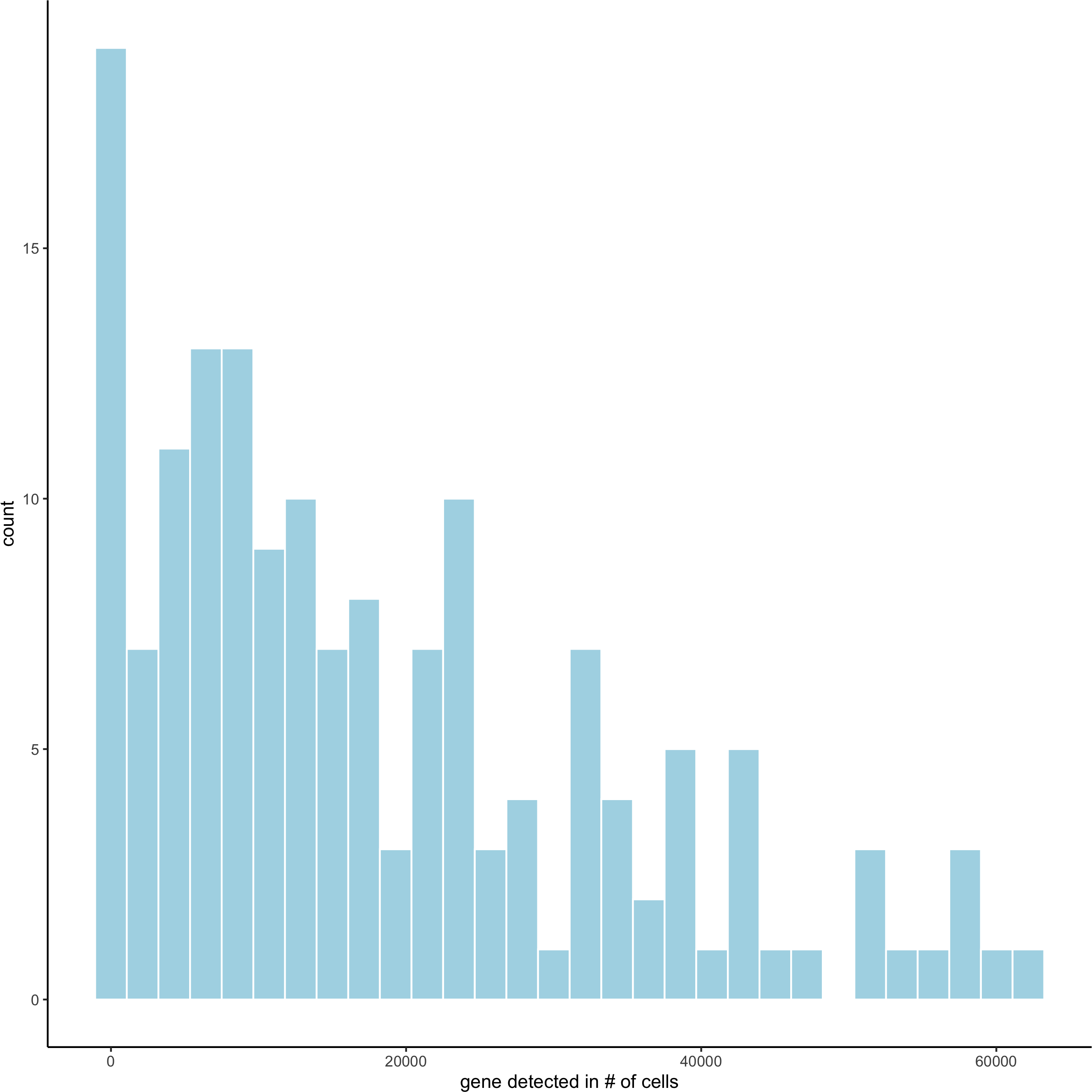
filterDistributions(merFISH_test, detection = 'genes',save_param = list(save_name = '2_a_distribution_genes'))

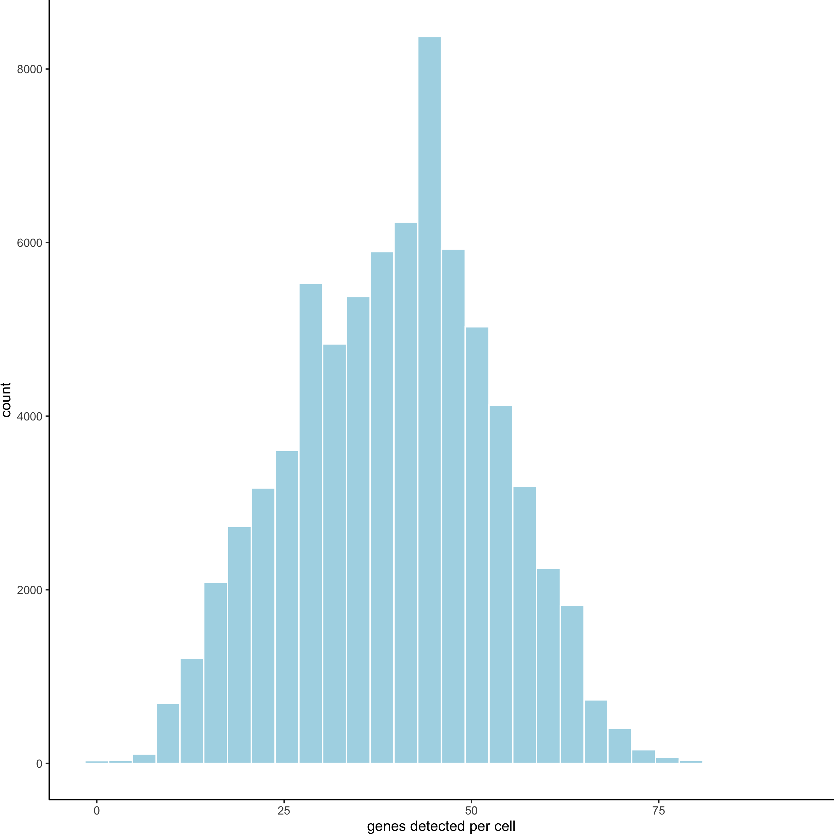
filterDistributions(merFISH_test, detection = 'cells',save_param = list(save_name = '2_b_distribution_cells'))

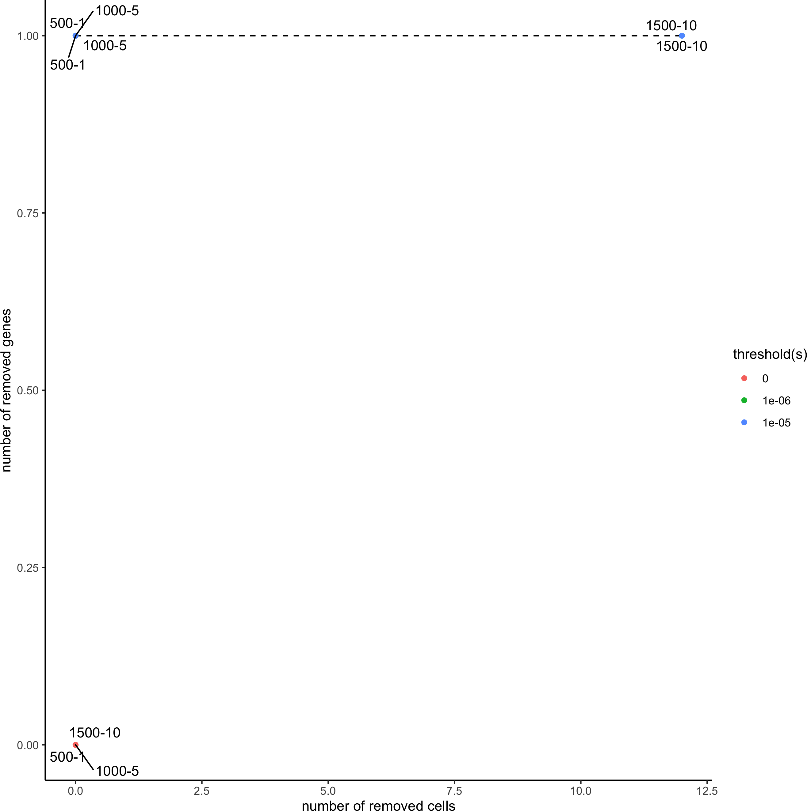
filterCombinations(merFISH_test,expression_thresholds = c(0,1e-6,1e-5),gene_det_in_min_cells = c(500, 1000, 1500),min_det_genes_per_cell = c(1, 5, 10), 
save_param = list(save_name = '2_c_filter_combos'))

# 2. filter data
merFISH_test <- filterGiotto(gobject = merFISH_test,gene_det_in_min_cells = 0,min_det_genes_per_cell = 0)
## normalize
merFISH_test <- normalizeGiotto(gobject = merFISH_test, scalefactor = 10000, verbose = T)
merFISH_test <- addStatistics(gobject = merFISH_test)
merFISH_test <- adjustGiottoMatrix(gobject = merFISH_test, expression_values = c('normalized'),batch_columns = NULL, covariate_columns = c('nr_genes', 'total_expr'),return_gobject = TRUE,update_slot = c('custom'))
# save according to giotto instructions
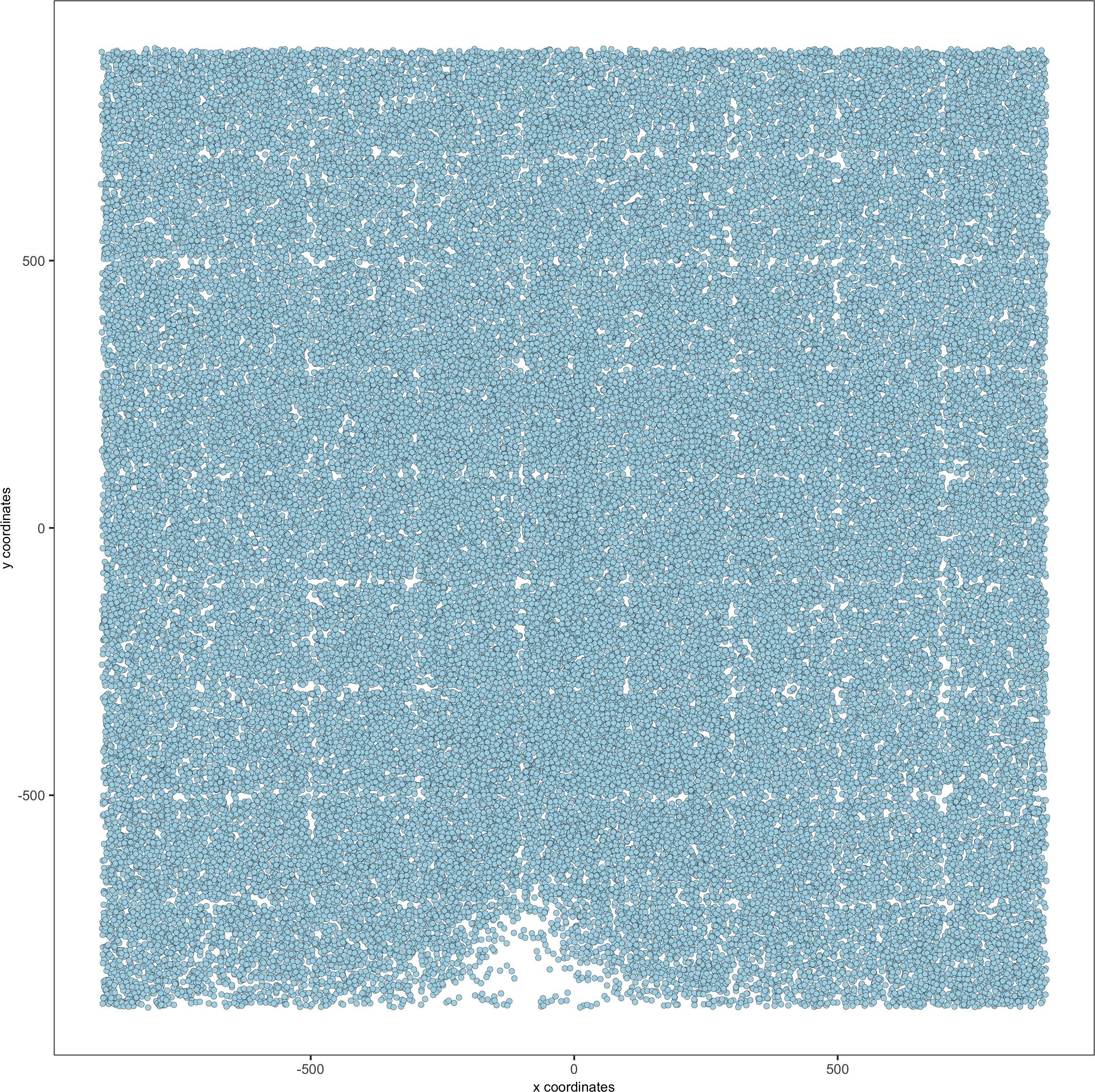
# 2D
spatPlot(gobject = merFISH_test, point_size = 1.5, 
save_param = list(save_name = '2_d_spatial_locations2D'))

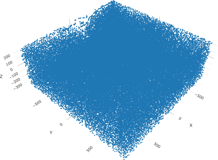
# 3D
spatPlot3D(gobject = merFISH_test, point_size = 2.0, axis_scale = 'real',save_param = list(save_name = '2_e_spatial_locations3D'))

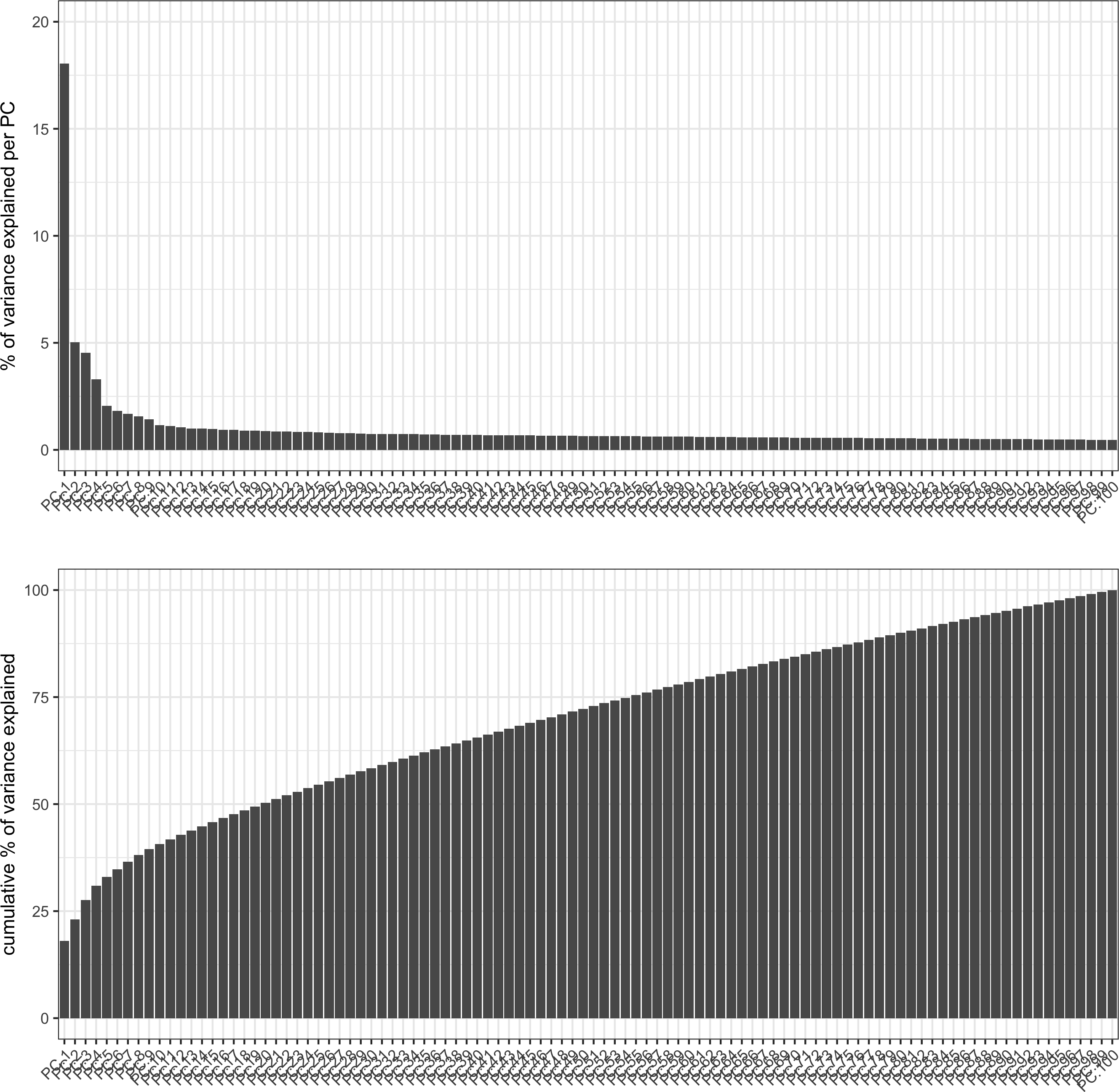
3. Dimension reduction

# only 155 genes, use them all (default)
merFISH_test <- runPCA(gobject = merFISH_test, genes_to_use = NULL, scale_unit = FALSE, center = TRUE)
screePlot(merFISH_test, save_param = list(save_name = '3_a_screeplot'))

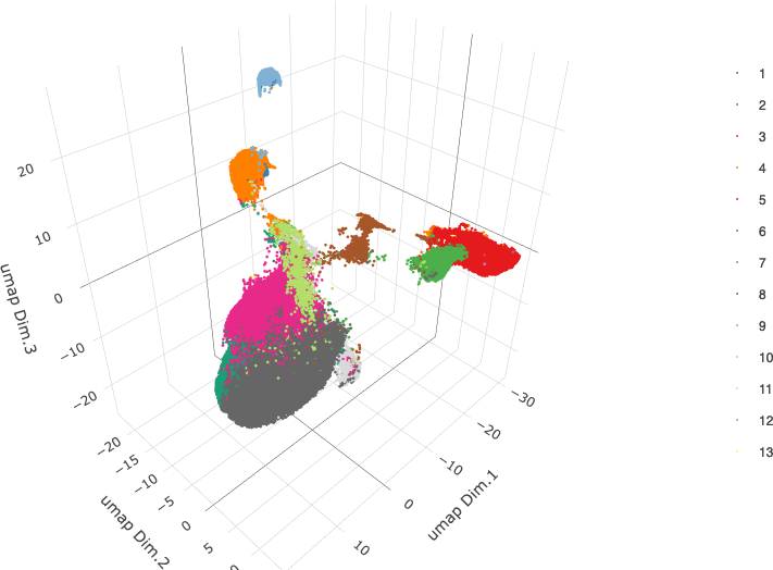
merFISH_test <- runUMAP(merFISH_test, dimensions_to_use = 1:8, n_components = 3, n_threads = 4)

plotUMAP_3D(gobject = merFISH_test, point_size = 1.5,save_param = list(save_name = '3_b_UMAP_reduction'))

4. Clustering

## sNN network (default)
merFISH_test <- createNearestNetwork(gobject = merFISH_test, dimensions_to_use = 1:8, k = 15)
## Leiden clustering
merFISH_test <- doLeidenCluster(gobject = merFISH_test, resolution = 0.2, n_iterations = 200,name = 'leiden_0.2')
plotUMAP_3D(gobject = merFISH_test, cell_color = 'leiden_0.2', point_size = 1.5, show_center_label = F,save_param = list(save_name = '4_a_UMAP_leiden'))

5. Co-visualize

spatDimPlot3D(gobject = merFISH_test, show_center_label = F,cell_color = 'leiden_0.2', dim3_to_use = 3,axis_scale = 'real', spatial_point_size = 2.0,save_param = list(save_name = '5_a_covis_leiden'))

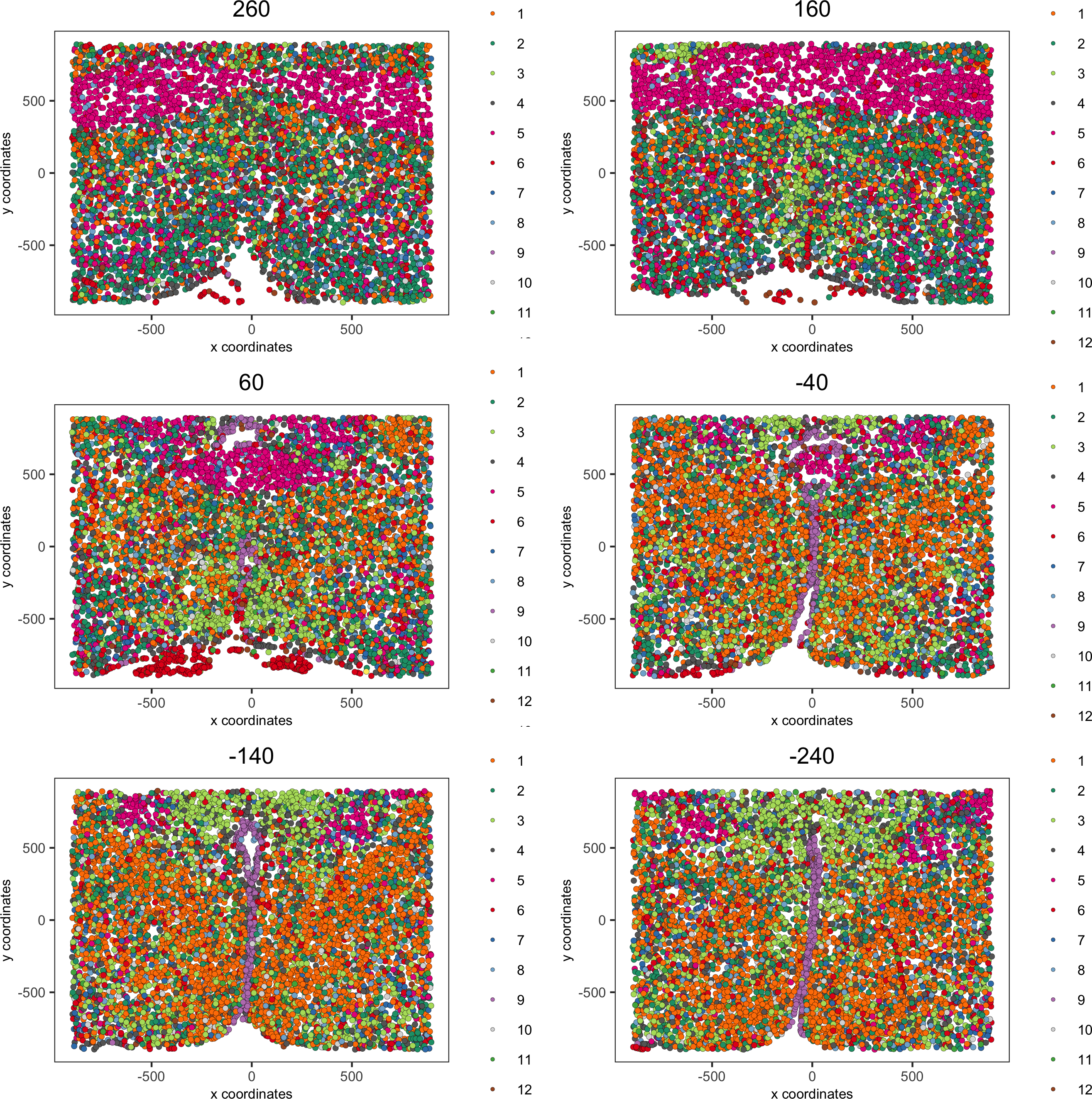
spatPlot2D(gobject = merFISH_test, point_size = 1.5, 
cell_color = 'leiden_0.2', 
group_by = 'layer_ID', cow_n_col = 2, group_by_subset = c(260, 160, 60, -40, -140, -240),save_param = list(save_name = '5_b_leiden_2D'))

6. Cell type marker gene detection

markers = findMarkers_one_vs_all(gobject = merFISH_test,method = 'gini',expression_values = 'normalized',cluster_column = 'leiden_0.2',min_genes = 1, rank_score = 2)
markers[, head(.SD, 2), by = 'cluster']

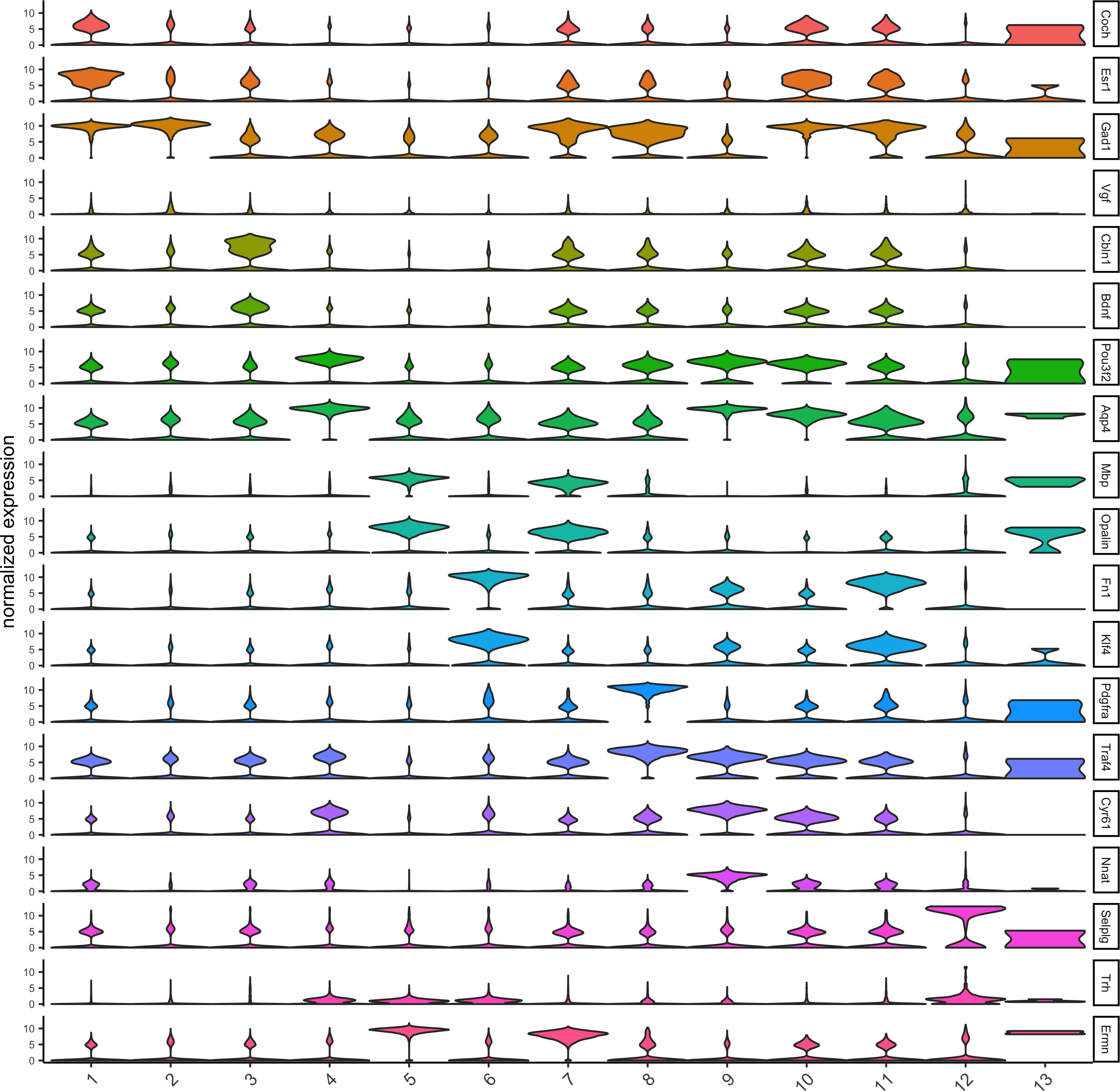
# violinplot
topgini_genes = unique(markers[, head(.SD, 2), by = 'cluster']$genes)
violinPlot(merFISH_test, genes = topgini_genes, cluster_column = 'leiden_0.2', strip_position = 'right',save_param = c(save_name = '6_a_violinplot'))

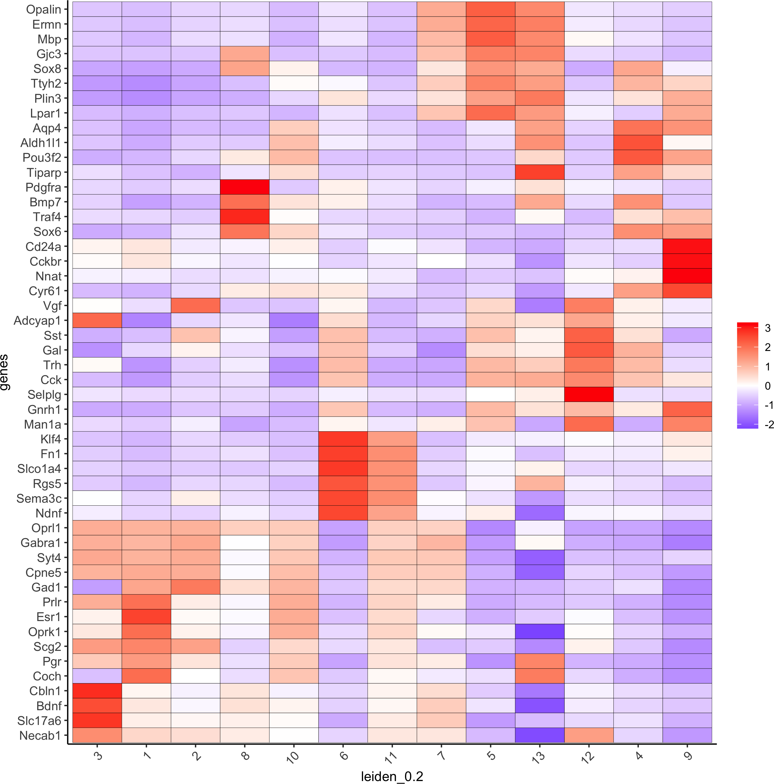
topgini_genes = unique(markers[, head(.SD, 6), by = 'cluster']$genes)
plotMetaDataHeatmap(merFISH_test, expression_values = 'scaled',metadata_cols = c('leiden_0.2'),selected_genes = topgini_genes,save_param = c(save_name = '6_b_clusterheatmap_markers'))

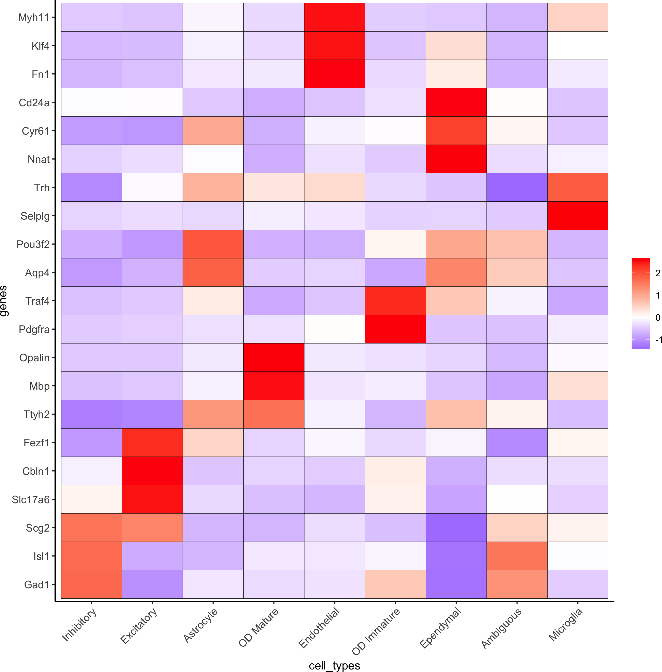
7. Cell-type annotation

7.1. Annotation

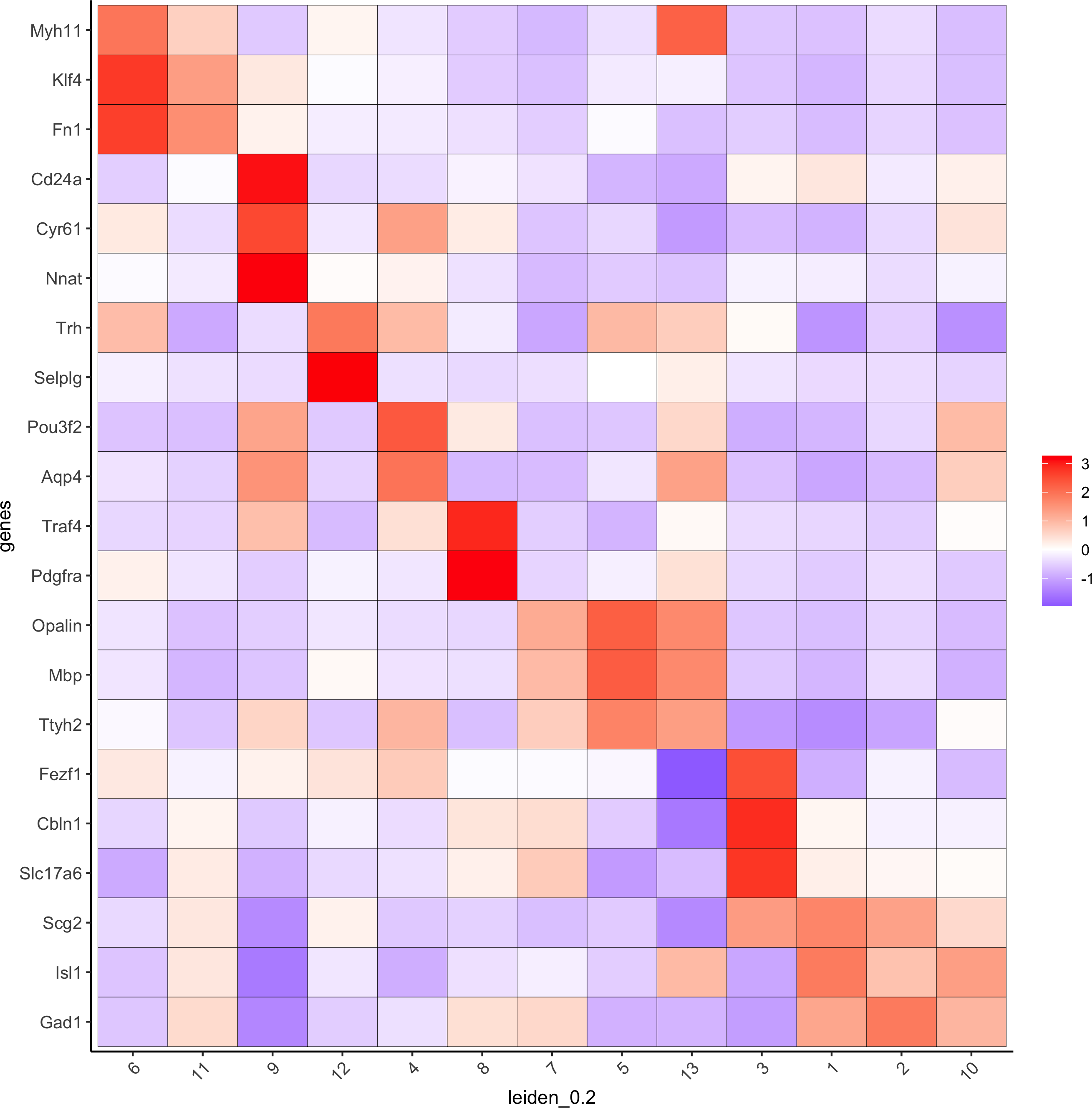
# known markers and DEGs
selected_genes = c('Myh11', 'Klf4', 'Fn1', 'Cd24a', 'Cyr61', 'Nnat', 'Trh', 'Selplg', 'Pou3f2', 'Aqp4', 'Traf4','Pdgfra', 'Opalin', 'Mbp', 'Ttyh2', 'Fezf1', 'Cbln1', 'Slc17a6', 'Scg2', 'Isl1', 'Gad1')
cluster_order = c(6, 11, 9, 12, 4, 8, 7, 5, 13, 3, 1, 2, 10)

plotMetaDataHeatmap(merFISH_test, expression_values = 'scaled',metadata_cols = c('leiden_0.2'),selected_genes = selected_genes,custom_gene_order = rev(selected_genes),custom_cluster_order = cluster_order,save_param = c(save_name = '7_a_clusterheatmap_markers'))

## name clusters
clusters_cell_types_hypo = c('Inhibitory', 'Inhibitory', 'Excitatory', 'Astrocyte','OD Mature', 'Endothelial','OD Mature', 'OD Immature', 'Ependymal', 'Ambiguous', 'Endothelial', 'Microglia', 'OD Mature')
names(clusters_cell_types_hypo) = as.character(sort(cluster_order))
merFISH_test = annotateGiotto(gobject = merFISH_test, annotation_vector = clusters_cell_types_hypo,cluster_column = 'leiden_0.2', name = 'cell_types')

## show heatmap
plotMetaDataHeatmap(merFISH_test, expression_values = 'scaled',metadata_cols = c('cell_types'),selected_genes = selected_genes,custom_gene_order = rev(selected_genes),custom_cluster_order = clusters_cell_types_hypo,save_param = c(save_name = '7_b_clusterheatmap_markers_celltypes'))

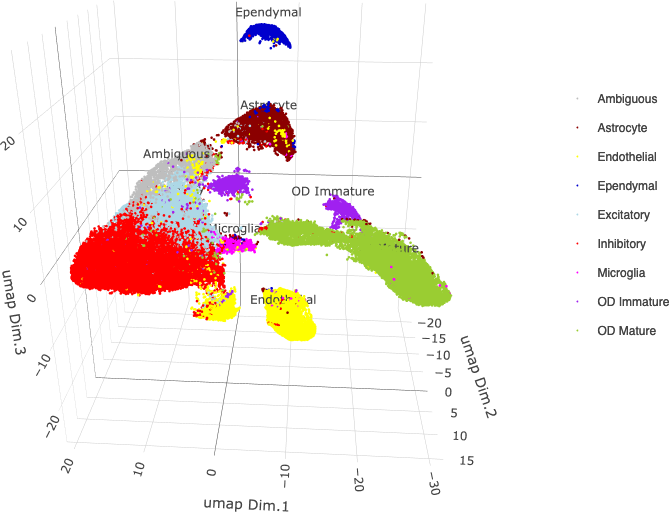
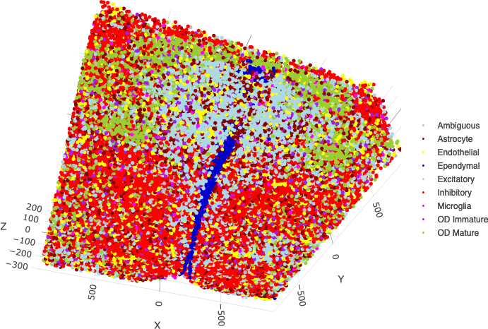
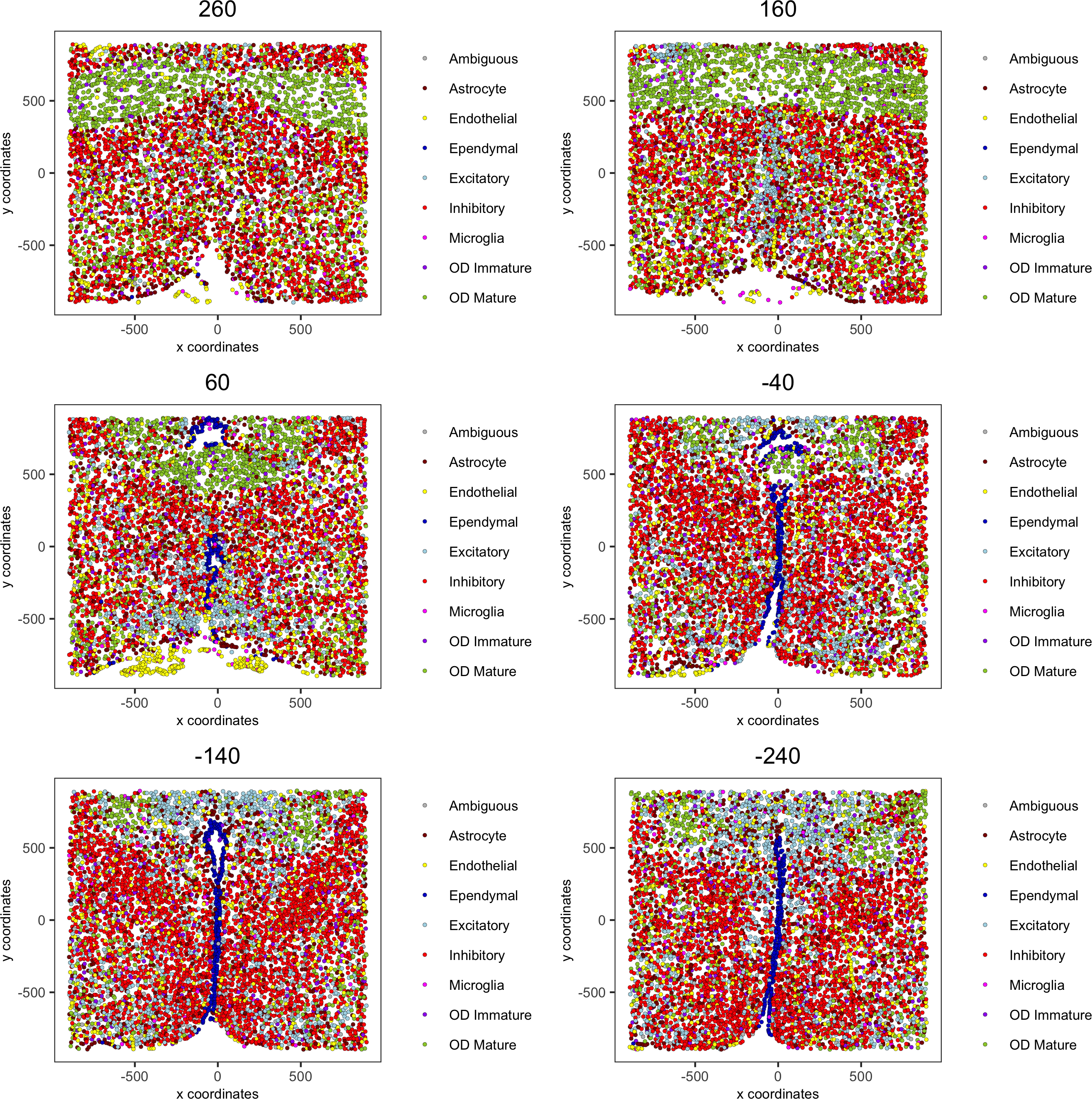
8. Visualization

## visualize ##
mycolorcode = c('red', 'lightblue', 'yellowgreen','purple', 'darkred', 'magenta', 'mediumblue', 'yellow', 'gray')
names(mycolorcode) = c('Inhibitory', 'Excitatory','OD Mature', 'OD Immature', 'Astrocyte', 'Microglia', 'Ependymal','Endothelial', 'Ambiguous')
plotUMAP_3D(merFISH_test, cell_color = 'cell_types', point_size = 1.5, cell_color_code = mycolorcode,save_param = c(save_name = '7_c_umap_cell_types'))

spatPlot3D(merFISH_test,cell_color = 'cell_types', axis_scale = 'real',sdimx = 'sdimx', sdimy = 'sdimy', sdimz = 'sdimz',show_grid = F, cell_color_code = mycolorcode,save_param = c(save_name = '7_d_spatPlot_cell_types_all'))

spatPlot2D(gobject = merFISH_test, point_size = 1.0,cell_color = 'cell_types', cell_color_code = mycolorcode,group_by = 'layer_ID', cow_n_col = 2, group_by_subset = c(seq(260, -290, -100)),save_param = c(save_name = '7_e_spatPlot2D_cell_types_all'))

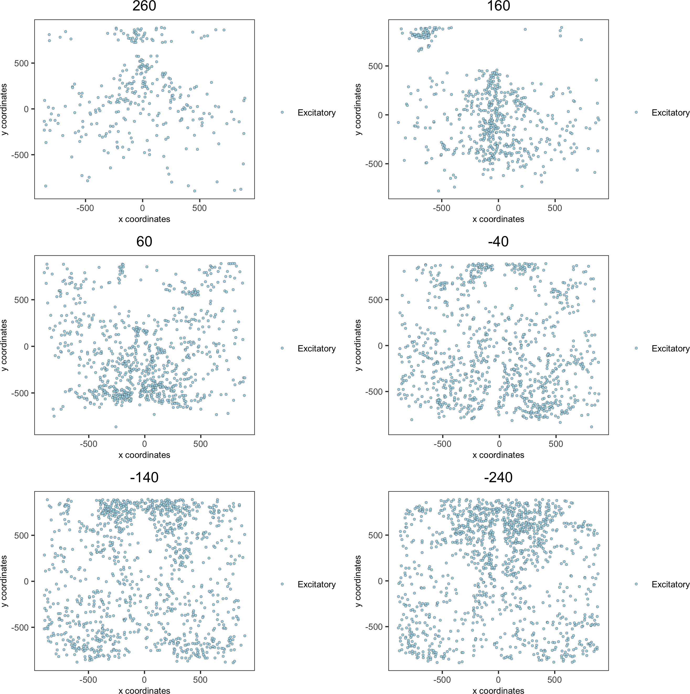
8.1 Excitatory cells only

spatPlot3D(merFISH_test,cell_color = 'cell_types', axis_scale = 'real',sdimx = 'sdimx', sdimy = 'sdimy', sdimz = 'sdimz',show_grid = F, cell_color_code = mycolorcode,select_cell_groups = 'Excitatory', show_other_cells = F,save_param = c(save_name = '7_f_spatPlot_cell_types_excit'))

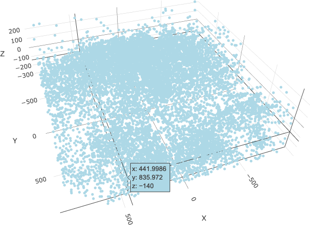
spatPlot2D(gobject = merFISH_test, point_size = 1.0, 
cell_color = 'cell_types', cell_color_code = mycolorcode,select_cell_groups = 'Excitatory', show_other_cells = F,group_by = 'layer_ID', cow_n_col = 2, group_by_subset = c(seq(260, -290, -100)),save_param = c(save_name = '7_g_spatPlot2D_cell_types_excit'))

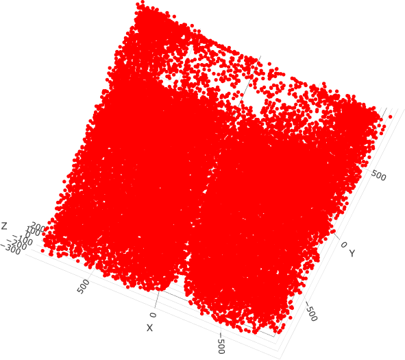
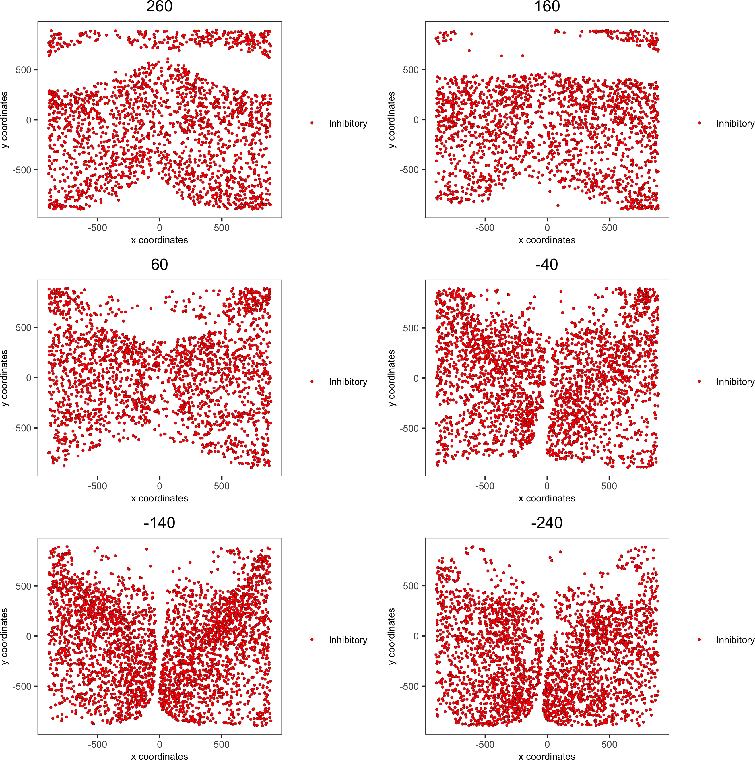
8.2 Inhibitory cells only

# inhibitory
spatPlot3D(merFISH_test,cell_color = 'cell_types', axis_scale = 'real',sdimx = 'sdimx', sdimy = 'sdimy', sdimz = 'sdimz',show_grid = F, cell_color_code = mycolorcode,select_cell_groups = 'Inhibitory', show_other_cells = F,save_param = c(save_name = '7_h_spatPlot_cell_types_inhib'))

spatPlot2D(gobject = merFISH_test, point_size = 1.0, 
cell_color = 'cell_types', cell_color_code = mycolorcode,select_cell_groups = 'Inhibitory', show_other_cells = F,group_by = 'layer_ID', cow_n_col = 2, group_by_subset = c(seq(260, -290, -100)),save_param = c(save_name = '7_i_spatPlot2D_cell_types_inhib'))

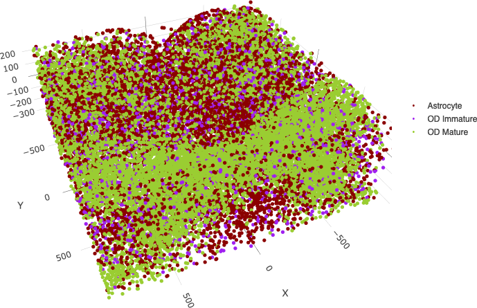
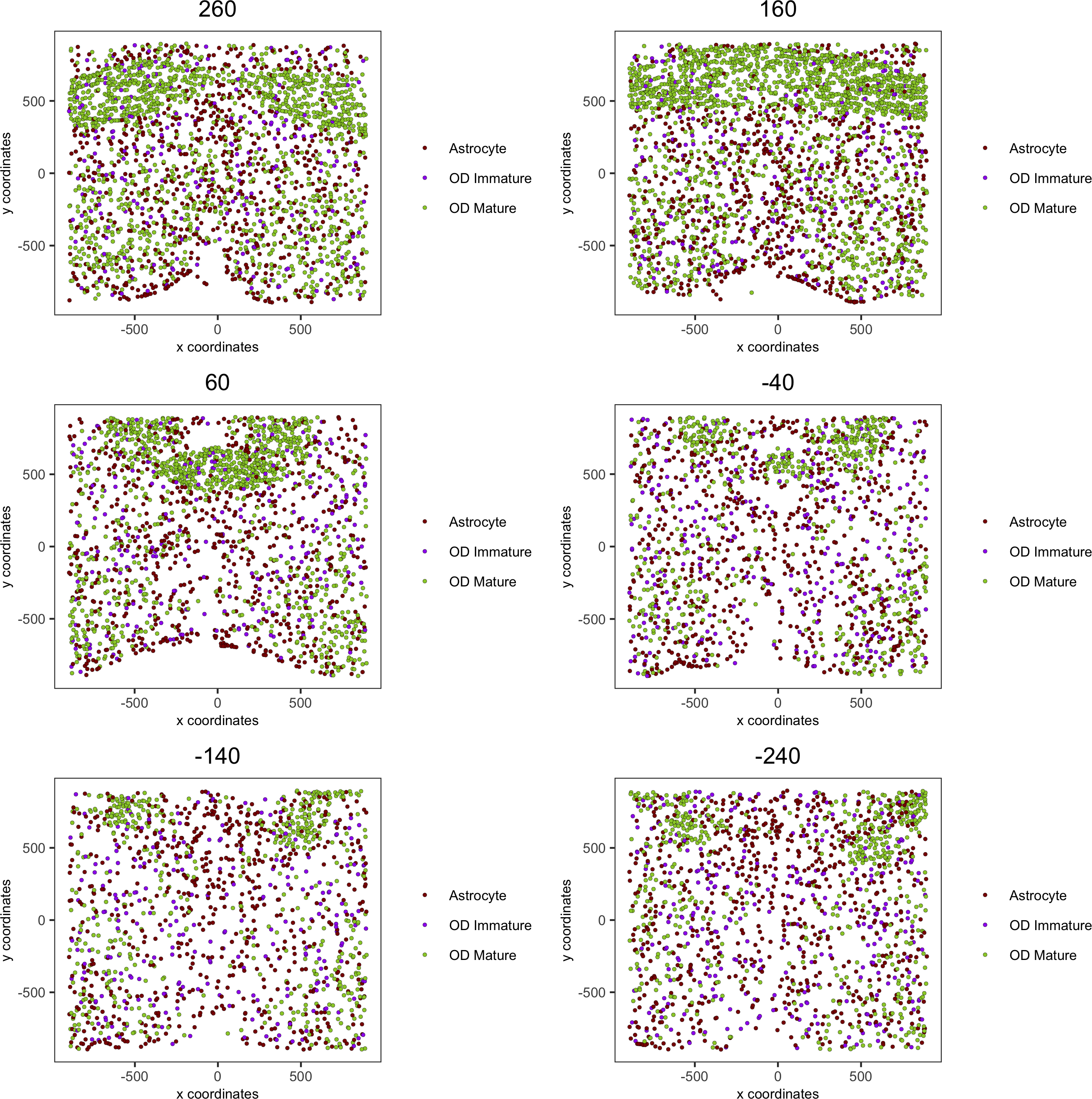
8.3 OD and astrocytes only

spatPlot3D(merFISH_test,cell_color = 'cell_types', axis_scale = 'real',sdimx = 'sdimx', sdimy = 'sdimy', sdimz = 'sdimz',show_grid = F, cell_color_code = mycolorcode,select_cell_groups = c('Astrocyte', 'OD Mature', 'OD Immature'), show_other_cells = F,save_param = c(save_name = '7_j_spatPlot_cell_types_ODandAstro'))

spatPlot2D(gobject = merFISH_test, point_size = 1.0, 
cell_color = 'cell_types', cell_color_code = mycolorcode,select_cell_groups = c('Astrocyte', 'OD Mature', 'OD Immature'), show_other_cells = F,group_by = 'layer_ID', cow_n_col = 2, group_by_subset = c(seq(260, -290, -100)),save_param = c(save_name = '7_k_spatPlot2D_cell_types_ODandAstro'))

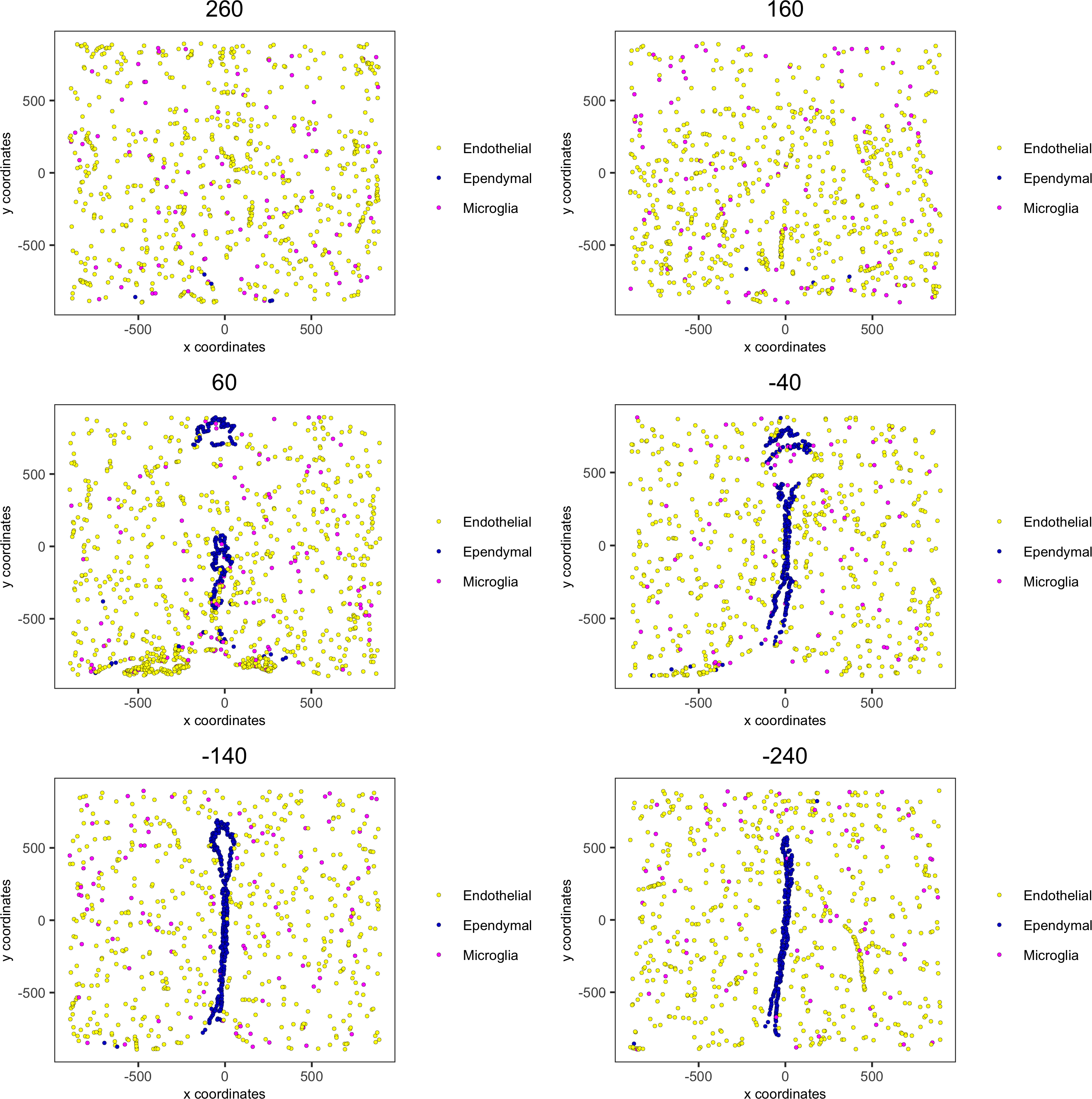
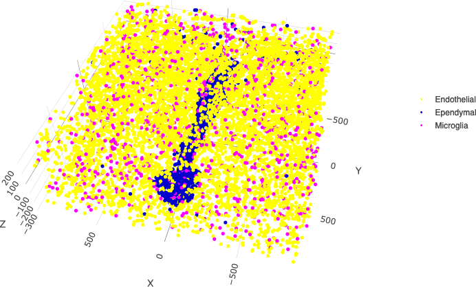
8.4 Other cells only

spatPlot3D(merFISH_test,cell_color = 'cell_types', axis_scale = 'real',sdimx = 'sdimx', sdimy = 'sdimy', sdimz = 'sdimz',show_grid = F, cell_color_code = mycolorcode,select_cell_groups = c('Microglia', 'Ependymal', 'Endothelial'), show_other_cells = F,save_param = c(save_name = '7_l_spatPlot_cell_types_other'))

spatPlot2D(gobject = merFISH_test, point_size = 1.0, 
cell_color = 'cell_types', cell_color_code = mycolorcode,select_cell_groups = c('Microglia', 'Ependymal', 'Endothelial'), show_other_cells = F,group_by = 'layer_ID', cow_n_col = 2, group_by_subset = c(seq(260, -290, -100)),save_param = c(save_name = '7_m_spatPlot2D_cell_types_other'))